GRaNIE Workflow Example
Christian Arnold
16 August 2023
GRaNIE_workflow.RmdAbstract
In this vignette, we present GRaNIE (Gene
Regulatory
Network Inference including
Enhancers), a framework to reconstruct predictive
enhancer-mediated regulatory network models that are based on
integrating of expression and chromatin accessibility/activity
pattern across individuals, and provide a comprehensive resource
of cell-type specific gene regulatory networks for particular cell
types. For an extended biological motivation, see the first
section below. In the following, we summarize how to use the
GRaNIE package in a real-world example, illustrate
most features and how to work with a GRaNIE object.
Importantly, this vignette will be continuously updated whenever
new functionality becomes available or when we receive user
feedback.
Motivation and Summary
Genetic variants associated with diseases often affect non-coding
regions, thus likely having a regulatory role. To understand the effects
of genetic variants in these regulatory regions, identifying genes that
are modulated by specific regulatory elements (REs) is crucial. The
effect of gene regulatory elements, such as enhancers, is often
cell-type specific, likely because the combinations of transcription
factors (TFs) that are regulating a given enhancer have cell-type
specific activity. This TF activity can be quantified with existing
tools such as diffTF and captures differences in binding of
a TF in open chromatin regions. Collectively, this forms a
enhancer-mediated gene regulatory network (eGRN) with
cell-type and data-specific TF-RE and RE-gene links. Here, we
reconstruct such a eGRN using bulk RNA-seq and open
chromatin (e.g., using ATAC-seq or ChIP-seq for open chromatin marks)
and optionally TF activity data. Our network contains different types of
links, connecting TFs to regulatory elements, the latter of which is
connected to genes in the vicinity or within the same chromatin domain
(TAD). We use a statistical framework to assign empirical FDRs
and weights to all links using a background-based approach.
For a more detailed description of the package, its mode of action, guidelines, recommendations, limitations, scope, etc,please see the Package Details Vignette on the GRaNIE website.
Example data
Before we start with the package, let’s retrieve some example data!
For the purpose of this vignette, the data we will use is taken from here 1,
has been minimally processed to meet the requirements of the
GRaNIE package and consists of the following files:
- ATAC-seq peaks, raw counts (originally around 75,000, genome-wide, here filtered to around 60,500)
- RNA-Seq data, raw counts (originally for around 35,000 genes, here filtered to around 19,000)
- sample metadata with additional sample-specific information
In general, the dataset is from human macrophages (both naive and
IFNg primed) of healthy individuals and various stimulations /
infections (naive vs primed and infected with SL1344 vs not), with 4
groups in total: control/infected(SL1344) and naive/primed(IFNg).
However, here for the example data, all ~30 samples are from IFNg primed
and infected cells (as summarized as IFNg_SL1344 in the
sample metadata column condition).
Furthermore, the example dataset is accompanied by the following files:
- genome-wide transcription factor binding site predictions for 6
selected TFs, along with a translation table to link TF names to their
corresponding Ensembl IDs. For each TF, a gzipped BED file has been
created with predicted TF binding sites. The files have been generated
with
PWMScanand theHOCOMOCOdatabase, see 2 for details.
Example Workflow
In the following example, you will use the example data to construct
a eGRN from ATAC-seq, RNA-seq data as well transcription
factor (TF) data.
First, let’s load the required libraries. The readr
package is already loaded and attached when loading the
GRaNIE package, but we nevertheless load it here explicitly
to highlight that we’ll use various `readr`` functions for data
import.
For reasons of brevity, we omit the output of this code chunk.
Install suggested, additional packages for full functionality
When installing GRaNIE, all required dependency packages are
automatically installed. In addition, GRaNIE needs some
additional packages for special functionality, packages that are not
strictly necessary for the workflow but which enhance the functionality,
may be required depending on certain parameters (such as your genome
assembly version), or may be required only when using a particular
functionality (such as the WGCNA package for a more robust
correlation method called bicor that is based on medians). The
package will automatically check if any of these packages are missing
during execution, and inform the user when a package is missing, along
with a line to copy for pasting into R for installation.
Note on version compatibility and errors in the vignette
We are actively working on the package and regularly improve upon features, add features, or change features for increased clarity. This sometimes results in minor changes to the workflow, changed argument names or other small incompatibilities that may result in errors when running a version of the package that differs from the version this vignette has been run for.
Thus, make sure to run a version of GRaNIE that
is compatible with this vignette. If in doubt or when you receive
errors, check the R help, which always contains the most up-to-date
documentation.
General notes
Each of the GRaNIE functions we mention here in this
Vignette comes with sensible default parameters that we found to work
well for most of the datasets we tested it with so far. For the purpose
of this Vignette, however, and the resulting running times, we here try
to provide a good compromise between biological necessity and
computational efficacy. However, always check the validity and
usefulness of the parameters before starting an analysis to
avoid unreasonable results.
Also, always check the Package Details Vignette, all methdological details are in there, and we regularly update it.
Reading the data required for the GRaNIE package
To set up a GRaNIE analysis, we first need to read in
some data into R.
For a more detailed description and list of the required and optional input data, please see the Package Details Vignette on the GRaNIE website.
Briefly, the following data can be used for the GRaNIE
package:
- open chromatin / peak data (from either ATAC-Seq, DNAse-Seq or ChIP-Seq data, for example), hereafter simply referred to as enhancers
- RNA-Seq data (gene expression counts for genes across samples)
The following data can be used optionally but are not required:
- sample metadata (e.g., sex, gender, age, sequencing batch, etc)
- TAD domains (bed file, not used here in this vignette)
So, let’s import the enhancer and RNA-seq data as a data frame as well as some sample metadata. This can be done in any way you want as long as you end up with the right format.
# We load the example data directly from the web:
file_peaks = "https://www.embl.de/download/zaugg/GRaNIE/countsATAC.filtered.tsv.gz"
file_RNA = "https://www.embl.de/download/zaugg/GRaNIE/countsRNA.filtered.tsv.gz"
file_sampleMetadata = "https://www.embl.de/download/zaugg/GRaNIE/sampleMetadata.tsv.gz"

countsRNA.df = read_tsv(file_RNA, col_types = cols())
countsPeaks.df = read_tsv(file_peaks, col_types = cols())
sampleMetadata.df = read_tsv(file_sampleMetadata, col_types = cols())


# Let's check how the data looks like
countsRNA.df
countsPeaks.df
sampleMetadata.df

# Save the name of the respective ID columns
idColumn_peaks = "peakID"
idColumn_RNA = "ENSEMBL"
## # A tibble: 18,972 × 30
## ENSEMBL babk_D bima_D cicb_D coyi_D diku_D eipl_D eiwy_D eofe_D fafq_D febc_D
## <chr> <dbl> <dbl> <dbl> <dbl> <dbl> <dbl> <dbl> <dbl> <dbl> <dbl>
## 1 ENSG00… 48933 48737 60581 93101 84980 91536 85728 35483 69674 58890
## 2 ENSG00… 49916 44086 50706 55893 57239 76418 75934 27926 57526 50491
## 3 ENSG00… 281733 211703 269460 239116 284509 389989 351867 164615 257471 304203
## 4 ENSG00… 98943 77503 92402 80927 96690 138149 115875 64368 91627 100039
## 5 ENSG00… 14749 15571 16540 16383 16886 21892 18045 10026 14663 15830
## 6 ENSG00… 64459 63734 71317 69612 72097 100487 78536 38572 65446 76910
## 7 ENSG00… 57449 55736 70798 66334 66424 91801 94729 40413 56916 66382
## 8 ENSG00… 15451 15570 15534 15945 10583 22601 16086 9275 16092 15291
## 9 ENSG00… 18717 18757 20051 18066 19648 28572 25240 11258 17739 20347
## 10 ENSG00… 168054 147822 178164 154220 168837 244731 215862 89368 158845 180734
## # … with 18,962 more rows, and 19 more variables: fikt_D <dbl>, guss_D <dbl>,
## # hayt_D <dbl>, hehd_D <dbl>, heja_D <dbl>, hiaf_D <dbl>, iill_D <dbl>,
## # kuxp_D <dbl>, nukw_D <dbl>, oapg_D <dbl>, oevr_D <dbl>, pamv_D <dbl>,
## # pelm_D <dbl>, podx_D <dbl>, qolg_D <dbl>, sojd_D <dbl>, vass_D <dbl>,
## # xugn_D <dbl>, zaui_D <dbl>
## # A tibble: 60,698 × 32
## peakID babk_D bima_D cicb_D coyi_D diku_D eipl_D eiwy_D eofe_D fafq_D febc_D
## <chr> <dbl> <dbl> <dbl> <dbl> <dbl> <dbl> <dbl> <dbl> <dbl> <dbl>
## 1 chrX:1… 3 7 10 5 4 6 3 18 4 22
## 2 chr15:… 5 28 38 11 20 19 7 53 5 22
## 3 chr12:… 5 14 18 5 3 13 5 15 2 25
## 4 chr1:1… 12 21 36 6 20 29 12 44 2 105
## 5 chr16:… 3 17 16 9 8 16 6 28 3 33
## 6 chr17:… 4 11 6 3 0 3 2 9 1 14
## 7 chr13:… 10 34 44 12 31 29 9 22 5 82
## 8 chr1:2… 21 113 46 28 44 57 47 146 12 91
## 9 chr14:… 5 9 14 6 6 9 8 16 2 26
## 10 chr8:1… 6 4 10 5 8 12 2 5 1 21
## # … with 60,688 more rows, and 21 more variables: fikt_D <dbl>, guss_D <dbl>,
## # hayt_D <dbl>, hehd_D <dbl>, heja_D <dbl>, hiaf_D <dbl>, iill_D <dbl>,
## # kuxp_D <dbl>, nukw_D <dbl>, oapg_D <dbl>, oevr_D <dbl>, pamv_D <dbl>,
## # pelm_D <dbl>, podx_D <dbl>, qolg_D <dbl>, sojd_D <dbl>, vass_D <dbl>,
## # xugn_D <dbl>, zaui_D <dbl>, uaqe_D <dbl>, qaqx_D <dbl>
## # A tibble: 31 × 16
## sample…¹ assig…² assig…³ atac_date clone condi…⁴ diff_start donor EB_forma…⁵
## <chr> <dbl> <dbl> <date> <dbl> <chr> <date> <chr> <date>
## 1 babk_D 5.51e6 0.211 2015-12-04 2 IFNg_S… 2015-10-12 babk 2015-10-09
## 2 bima_D 2.33e7 0.677 2014-12-12 1 IFNg_S… 2014-11-07 bima 2014-11-04
## 3 cicb_D 1.98e7 0.580 2015-04-24 3 IFNg_S… 2015-03-30 cicb 2015-03-27
## 4 coyi_D 6.73e6 0.312 2015-11-05 3 IFNg_S… 2015-09-30 coyi 2015-09-27
## 5 diku_D 7.01e6 0.195 2015-11-13 1 IFNg_S… 2015-10-15 diku 2015-10-12
## 6 eipl_D 1.69e7 0.520 2015-08-04 1 IFNg_S… 2015-06-30 eipl 2015-06-27
## 7 eiwy_D 9.81e6 0.404 2015-12-02 1 IFNg_S… 2015-10-23 eiwy 2015-10-20
## 8 eofe_D 2.57e7 0.646 2014-12-12 1 IFNg_S… 2014-11-01 eofe 2014-10-29
## 9 fafq_D 4.60e6 0.415 2015-10-14 1 IFNg_S… 2015-09-16 fafq 2015-09-13
## 10 febc_D 3.17e7 0.430 2015-08-04 2 IFNg_S… 2015-07-06 febc 2015-07-03
## # … with 21 more rows, 7 more variables: macrophage_diff_days <dbl>,
## # medium_changes <dbl>, mt_frac <dbl>, percent_duplication <dbl>,
## # received_as <chr>, sex <chr>, short_long_ratio <dbl>, and abbreviated
## # variable names ¹sample_id, ²assigned, ³assigned_frac, ⁴condition,
## # ⁵EB_formationWhile we recommend raw counts for both enhancers and RNA-Seq as input
and offer several normalization choices in the pipeline, it is also
possible to provide pre-normalized data. Note that the normalization
method may have a large influence on the resulting eGRN
network, so make sure the choice of normalization is reasonable. For
more details, see the next sections.
As you can see, both enhancers and RNA-Seq counts must have exactly
one ID column, with all other columns being numeric. For enhancers, this
column may be called peakID, for example, but the exact
name is not important and can be specified as a parameter later when
adding the data to the object. The same applies for the RNA-Seq data,
whereas a sensible choice here is ensemblID, for
example.
For the enhancer ID column, the required format is
chr:start-end, with chr denoting the
chromosome, followed by “:”, and then start,
-, and end for the enhancer start and end,
respectively. As the coordinates for the enhancers are needed in the
pipeline, the format must be exactly as stated here.
You may notice that the enhancers and RNA-seq data have different
samples being included, and not all are overlapping. This is not a
problem and as long as some samples are found in both of them,
the GRaNIE pipeline can work with it. Note that only the
shared samples between both data modalities are kept, however, so make
sure that the sample names match between them and share as many samples
as possible.
Initialize a GRaNIE object
We got all the data in the right format, we can start with our
GRaNIE analysis now! We start by specifying some parameters
such as the genome assembly version the data have been produced with, as
well as some optional object metadata that helps us to distinguish this
GRaNIE object from others.
genomeAssembly = "hg38"  #Either hg19, hg38 or mm10. Both enhancers and RNA data must have the same genome assembly

# Optional and arbitrary list with information and metadata that is stored
# within the GRaNIE object
objectMetadata.l = list(name = paste0("Macrophages_infected_primed"), file_peaks = file_peaks,
    file_rna = file_RNA, file_sampleMetadata = file_sampleMetadata, genomeAssembly = genomeAssembly)

dir_output = "."

GRN = initializeGRN(objectMetadata = objectMetadata.l, outputFolder = dir_output,
    genomeAssembly = genomeAssembly)

GRN
## INFO [2023-08-16 17:37:50] Empty GRN object created successfully. Type the object name (e.g., GRN) to retrieve summary information about it at any time.
## INFO [2023-08-16 17:37:50] Default output folder: /g/zaugg/carnold/Projects/GRN_packages/GRaNIE/vignettes/
## INFO [2023-08-16 17:37:50] Genome assembly: hg38
## INFO [2023-08-16 17:37:50] Finished successfully. Execution time: 0.1 secs
## GRN object from package GRaNIE (created with version 1.5.2)
## Data summary:
## Peaks: No peak data found.
## Genes: No RNA-seq data found.
## TFs: No TF data found.
## Parameters:
## Output directory: /g/zaugg/carnold/Projects/GRN_packages/GRaNIE/vignettes/
## Provided metadata:
## name : Macrophages_infected_primed
## file_peaks : https://www.embl.de/download/zaugg/GRaNIE/countsATAC.filtered.tsv.gz
## file_rna : https://www.embl.de/download/zaugg/GRaNIE/countsRNA.filtered.tsv.gz
## file_sampleMetadata : https://www.embl.de/download/zaugg/GRaNIE/sampleMetadata.tsv.gz
## genomeAssembly : hg38
## Connections:
## TF-peak links: none found
## peak-gene links: none found
## TF-peak-gene links (filtered): none found
## Network-related:
## eGRN network: not foundInitializing a GRaNIE object occurs in the function
initializeGRN() and is trivial: All we need to specify is
an output folder (this is where all the pipeline output is automatically
being saved unless specified otherwise) and the genome assembly shortcut
of the data. We currently support hg19, hg38,
and mm10. Please contact us if you need additional genomes.
The objectMetadata argument is recommended but optional and
may contain an arbitrarily complex named list that is stored as
additional metadata for the GRaNIE object. Here, we decided
to specify a name for the GRaNIE object as well as the
original paths for all 3 input files and the genome assembly.
For more parameter details, see the R help
(?initializeGRN).
At any time point, we can simply “print” a GRaNIE object
by typing its name and a summary of the content is printed to the
console (as done above in the last line of the code block).
Add data
We are now ready to fill our empty object with data! After preparing
the data beforehand, we can now use the data import function
addData() to import both enhancers and RNA-seq data to the
GRaNIE object. In addition to the count tables, we
explicitly specify the name of the ID columns. As mentioned before, the
sample metadata is optional but recommended if available.
An important consideration is data normalization for RNA and ATAC. We
support many different choices of normalization, the selection of which
also depends on whether RNA or peaks is considered, and possible choices
are: limma_quantile, DESeq2_sizeFactors and
none and refer to the R help for more details
(?addData). The default for RNA-Seq is a quantile
normalization, while for the open chromatin enhancer data, it is
DESeq2_sizeFactors (i.e., a “regular” DESeq2
size factor normalization). Importantly, DESeq2_sizeFactors
requires raw data, while limma_quantile does not
necessarily. We nevertheless recommend raw data as input, although it is
also possible to provide pre-normalized data as input and then topping
this up with another normalization method or none.
GRN = addData(GRN, counts_peaks = countsPeaks.df, normalization_peaks = "DESeq2_sizeFactors",
    idColumn_peaks = idColumn_peaks, counts_rna = countsRNA.df, normalization_rna = "limma_quantile",
    idColumn_RNA = idColumn_RNA, sampleMetadata = sampleMetadata.df, forceRerun = TRUE)

GRN
Only overlapping samples between the two data modalities are kept in
the GRaNIE object. Here, all 29 samples from the RNA data
are kept because they are also found in the peak data, while only 29 out
of 31 samples from the peak data are also found in the RNA data,
resulting in 29 shared samples overall. The RNA counts are also
shuffled, which will be the basis for all analysis and plots in
subsequent steps that repeat the analysis for the background
eGRN in addition to the real one.
When we print the GRN object again, we see that the
added information from addData is now also printed in a
summarized manner.
Object history
The package also provides a history or
tracking function: In a GRN object, all previously
used function calls that modified the object are stored for user
convenience and reproducibility purposes.
For example, to retrieve the information about how the
addData function was used in the context of the
GRN object we have here, simply type
GRN@config$functionParameters$addData to retrieve a
(nested) list with all necessary details.
For more details, see the Package Details.
Quality control 1: PCA plots
It is time for our first QC plots using the function
plotPCA_all()! Now that we added peak and RNA data to the
object, let’s check with a Principal Component Analysis (PCA)
for both peak and RNA-seq data as well as the original input and the
normalized data (unless normalization has been set to none, in which
case they are identical to the original data) where the variation in the
data comes from. If sample metadata has been provided in the
addData() function (something we strongly recommend), they
are automatically added to the PCA plots by coloring the PCA results
according to the provided metadata, so that potential batch effects can
be examined and identified. For more details, see the R help
(?plotPCA_all).
Note that while this step is recommended to do, it is fully optional from a workflow point of view.
GRN = plotPCA_all(GRN, data = c("rna"), topn = 500, type = "normalized", plotAsPDF = FALSE,
    pages = c(2, 3, 14), forceRerun = TRUE)
Depending on the parameters, multiple output files (and plots) may be
produced, with up to two files for each of the specified
data modalities (that is, RNA-Seq counts, as specified with
rna here, as well as the peak counts, peaks,
not done here for reasons of brevity). For each of them, PCA plots can
be produced for both raw and normalized data
(here: only raw). With raw, we here denote the
original counts as given as input with the addData()
function, irrespective of whether this was already pre-normalized or
not. The topn argument specifies the number of top variable
features to do PCA for - here 500.
There are more plots that are generated, make sure to examine these plots closely! For all details, which plots are produced and further comments on how to understand and interpret them, see the Package Details.
Add TFs and TFBS and overlap with peak
Now it is time to add data for TFs and predicted TF binding sites
(TFBS)! Our GRaNIE package requires pre-computed TFBS that
need to be in a specific format. In brief, a 6-column bed file must be
present for each TF, with a specific file name that starts with the name
of the TF, an arbitrary and optional suffix (here: _TFBS)
and a particular file ending (supported are bed or
bed.gz; here, we specify the latter). All these files must
be located in a particular folder that the addTFBS()
functions then searches in order to identify those files that match the
specified patterns. We provide example TFBS for the 3 genome assemblies
we support. After setting this up, we are ready to overlap the TFBS and
the peaks by calling the function
overlapPeaksAndTFBS().
For more details how to download the full set of TF and TFBS data, see the Package Details.
For more parameter details, see the R help (?addTFBS and
?overlapPeaksAndTFBS).
folder_TFBS_6TFs = "https://www.embl.de/download/zaugg/GRaNIE/TFBS_selected.zip"
# Download the zip of all TFBS files. Takes too long here, not executed
# therefore

download.file(folder_TFBS_6TFs, file.path("TFBS_selected.zip"), quiet = FALSE)

unzip(file.path("TFBS_selected.zip"), overwrite = TRUE)

motifFolder = tools::file_path_as_absolute("TFBS_selected")

GRN = addTFBS(GRN, motifFolder = motifFolder, TFs = "all", filesTFBSPattern = "_TFBS",
    fileEnding = ".bed.gz", forceRerun = TRUE)

GRN = overlapPeaksAndTFBS(GRN, nCores = 1, forceRerun = TRUE)
We see from the output (omitted here for brevity) that 6 TFs have
been found in the specified input folder, and the number of TFBS that
overlap our peaks for each of them. We successfully added our TFs and
TFBS to the GRaNIE object”
Filter data (optional)
Optionally, we can filter both peaks and RNA-Seq data according to
various criteria using the function filterData().
For the open chromatin peaks, we currently support three filters:
- Filter by their normalized mean read counts
(
minNormalizedMean_peaks, default 5) - Filter by their size / width (in bp) and discarding peaks that
exceed a particular threshold (
maxSize_peaks, default: 10000 bp) - Filter by chromosome (only keep chromosomes that are provided as
input to the function,
chrToKeep_peaks)
For RNA-seq, we currently support the analogous filter as for open
chromatin for normalized mean counts as explained above
(minNormalizedMeanRNA).
The default values are usually suitable for bulk data and should result in the removal of very few peaks / genes; however, for single-cell data, lowering them may more reasonable. The output will print clearly how many peaks and genes have been filtered, so you can rerun the function with different values if needed.
For more parameter details, see the R help
(?filterData).
# Chromosomes to keep for peaks. This should be a vector of chromosome names
chrToKeep_peaks = c(paste0("chr", 1:22), "chrX")
GRN = filterData(GRN, minNormalizedMean_peaks = 5, minNormalizedMeanRNA = 1, chrToKeep_peaks = chrToKeep_peaks,
    maxSize_peaks = 10000, forceRerun = TRUE)
## INFO [2023-08-16 17:37:57] FILTER PEAKS
## INFO [2023-08-16 17:37:57] Number of peaks before filtering : 75000
## INFO [2023-08-16 17:37:57] Filter peaks by CV: Min = 0
## INFO [2023-08-16 17:37:57] Filter peaks by mean: Min = 5
## INFO [2023-08-16 17:37:57] Number of peaks after filtering : 64008
## INFO [2023-08-16 17:37:57] Finished successfully. Execution time: 0.1 secs
## INFO [2023-08-16 17:37:57] Filter and sort peaks by size and remain only those bigger than 20 and smaller than 10000
## INFO [2023-08-16 17:37:57] Filter and sort peaks and remain only those on the following chromosomes: chr1,chr2,chr3,chr4,chr5,chr6,chr7,chr8,chr9,chr10,chr11,chr12,chr13,chr14,chr15,chr16,chr17,chr18,chr19,chr20,chr21,chr22,chrX
## INFO [2023-08-16 17:37:57] Number of peaks before filtering: 75000
## INFO [2023-08-16 17:37:57] Number of peaks after filtering : 75000
## INFO [2023-08-16 17:37:57] Finished successfully. Execution time: 0.1 secs
## INFO [2023-08-16 17:37:58] Collectively, filter 10992 out of 75000 peaks.
## INFO [2023-08-16 17:37:58] Number of remaining peaks: 64008
## INFO [2023-08-16 17:37:59] FILTER RNA-seq
## INFO [2023-08-16 17:37:59] Number of genes before filtering : 61534
## INFO [2023-08-16 17:37:59] Filter genes by CV: Min = 0
## INFO [2023-08-16 17:37:59] Filter genes by mean: Min = 1
## INFO [2023-08-16 17:37:59] Number of genes after filtering : 18924
## INFO [2023-08-16 17:37:59] Finished successfully. Execution time: 0.1 secs
## INFO [2023-08-16 17:37:59] Flagged 16129 rows due to filtering criteria
## INFO [2023-08-16 17:37:59] Finished successfully. Execution time: 1.6 secsWe can see from the output that no peaks have been filtered due to their size and almost 11,000 have been filtered due to their small mean read counts, which collectively leaves around 64,000 peaks out of 75,000 originally. For the RNA data, almost half of the data has been filtered (16,211 out of around 35,000 genes).
Add TF-enhancer connections
We now have all necessary data in the object to start constructing
our network. As explained elsewhere, we currently support two types of
links for our GRaNIE approach:
- TF - peak/enhancer
- peak/enhancer - gene
Let’s start with TF-enhancer links! For this, we employ the function
addConnections_TF_peak(). By default, we use Pearson to
calculate the correlations between TF expression and enhancer
accessibility, but Spearman may sometimes be a better alternative,
especially if the diagnostic plots show that the background is not
looking as expected.
In addition to creating TF-enhancer links based on TF expression, we
can also correlate enhancer accessibility with other measures. We call
this the connection type, and expression is the
default one in our framework. However, we implemented a flexible way of
allowing also additional or other connection types. Briefly, this works
as follows: Additional data has to be imported beforehand with a
particular name (the name of the connection type). For example,
measures that are related to so-called TF activity can be used
in addition or as a replacement of TF expression. For each connection
type that we want to include, we simply add it to the parameter
connectionTypes along with the binary vector
removeNegativeCorrelation that specifies whether or not
negatively correlated pairs should be removed or not. For expression,
the default is to not remove them, while removal may be more reasonable
for measures related to TF activity (see here
for more details).
Lastly, we offer a so called GC-correction that uses a GC-matching background to compare it with the foreground instead of using the full background as comparison. For more details, see here. We are still investigating the plausibility and effects of this and therefore mark this feature as experimental as of now.
Note that the TF-enhancer links are constructed for both the original
data (in the corresponding output plots that are produced, this is
labeled as original) and the (shuffled) background
(background). For more methodological details, see the Package Details
Vignette. For more parameter options and details, see the R help
(?addConnections_TF_peak).
GRN = addConnections_TF_peak(GRN, plotDiagnosticPlots = FALSE, connectionTypes = c("expression"),
    corMethod = "pearson", forceRerun = TRUE)
## INFO [2023-08-16 17:37:59]
## Real data
##
## INFO [2023-08-16 17:37:59] Calculate TF-peak links for connection type expression
## INFO [2023-08-16 17:37:59] Correlate expression and peak counts
## INFO [2023-08-16 17:37:59] Retain 59 unique genes from TF/gene data out of 18904 (filter 18845 non-TF genes and 0 TF genes with 0 counts throughout).
## INFO [2023-08-16 17:37:59] Correlate TF/gene data for 59 unique Ensembl IDs (TFs) and peak counts for 64008 peaks.
## INFO [2023-08-16 17:37:59] Note: For subsequent steps, the same gene may be associated with multiple TF, depending on the translation table.
## INFO [2023-08-16 17:38:00] Finished successfully. Execution time: 0.5 secs
## INFO [2023-08-16 17:38:00] Run FDR calculations for 65 TFs for which TFBS predictions and expression data for the corresponding gene are available.
## INFO [2023-08-16 17:38:00] Skip the following 10 TF due to missing data or because they are marked as filtered: ATOH1.0.B,CDX1.0.C,CTCFL.0.A,DLX6.0.D,DMRT1.0.D,EHF.0.B,ESR2.0.A,ESR2.1.A,FOXA3.0.B,FOXB1.0.D
## INFO [2023-08-16 17:38:00] Compute FDR for each TF. This may take a while...
## INFO [2023-08-16 17:38:13] Finished successfully. Execution time: 14 secs
## INFO [2023-08-16 17:38:13] Finished successfully. Execution time: 14 secs
## INFO [2023-08-16 17:38:13] Finished. Stored 23096 connections with an FDR <= 0.3
## INFO [2023-08-16 17:38:13]
## Permuted data
##
## INFO [2023-08-16 17:38:13] Shuffling rows per column
## INFO [2023-08-16 17:38:14] Finished successfully. Execution time: 0.5 secs
## INFO [2023-08-16 17:38:14] Calculate TF-peak links for connection type expression
## INFO [2023-08-16 17:38:14] Correlate expression and peak counts
## INFO [2023-08-16 17:38:15] Retain 59 unique genes from TF/gene data out of 18904 (filter 18845 non-TF genes and 0 TF genes with 0 counts throughout).
## INFO [2023-08-16 17:38:15] Correlate TF/gene data for 59 unique Ensembl IDs (TFs) and peak counts for 64008 peaks.
## INFO [2023-08-16 17:38:15] Note: For subsequent steps, the same gene may be associated with multiple TF, depending on the translation table.
## INFO [2023-08-16 17:38:15] Finished successfully. Execution time: 0.4 secs
## INFO [2023-08-16 17:38:15] Run FDR calculations for 65 TFs for which TFBS predictions and expression data for the corresponding gene are available.
## INFO [2023-08-16 17:38:15] Skip the following 10 TF due to missing data or because they are marked as filtered: ATOH1.0.B,CDX1.0.C,CTCFL.0.A,DLX6.0.D,DMRT1.0.D,EHF.0.B,ESR2.0.A,ESR2.1.A,FOXA3.0.B,FOXB1.0.D
## INFO [2023-08-16 17:38:15] Compute FDR for each TF. This may take a while...
## INFO [2023-08-16 17:38:27] Finished successfully. Execution time: 12.9 secs
## INFO [2023-08-16 17:38:27] Finished successfully. Execution time: 13.5 secs
## INFO [2023-08-16 17:38:27] Finished. Stored 54 connections with an FDR <= 0.3
## INFO [2023-08-16 17:38:27] Finished successfully. Execution time: 27.7 secsFrom the output, we see that all of the 6 TFs also have RNA-seq data available and consequently will be included and correlated with the peak accessibility.
Quality control 2: Diagnostic plots for TF-enhancer connections
After adding the TF-enhancer links to our GRaNIE object,
let’s look at some diagnostic plots. Depending on the user parameters,
the plots are either directly plotted to the currently active graphics
device or to PDF files as specified in the object or via the function
parameters. If plotted to a PDF, within the specified or default output
folder (when initializing the GRaNIE object) should contain
two new files that are named TF_peak.fdrCurves_original.pdf
and TF_peak.fdrCurves_background.pdf, for example.
For real data and all TFs, this function may run a while, and each time-consuming step has a built-in progress bar for the plot-related parts so the remaining time can be estimated.
For reasons of brevity and organization, we fully describe their interpretation and meaning in detail in the Package Details Vignette.
In summary, we provide an overview of the total number of TF-peak connections for a range of typically used FDR values for both real and background TF-peak links, stratified by the TF-peak correlation bin
GRN = plotDiagnosticPlots_TFPeaks(GRN, dataType = c("real"), plotAsPDF = FALSE, pages = c(1))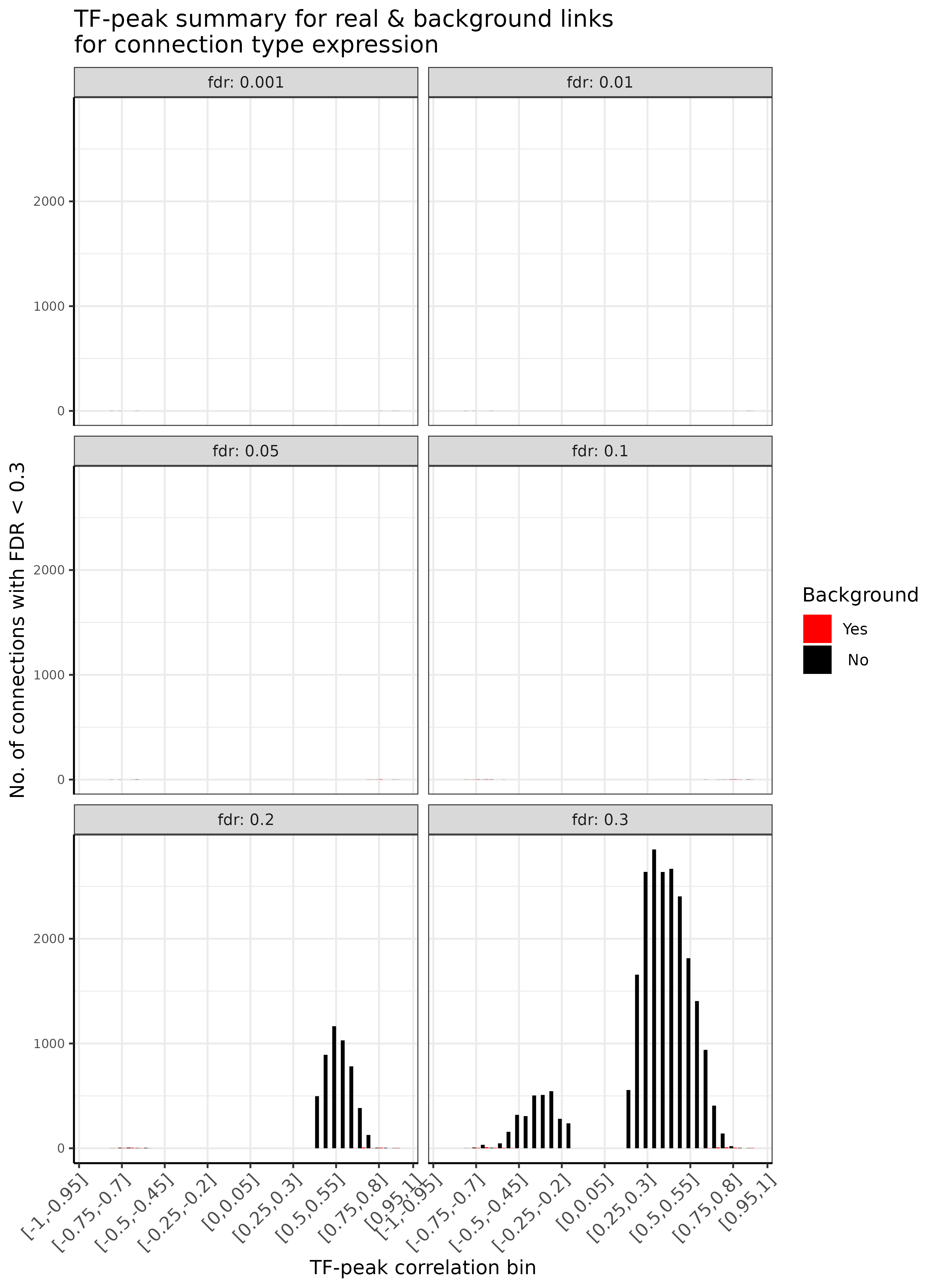
TF-enhancer diagnostic plots connection overview.A
## INFO [2023-08-16 17:38:27]
##  Plotting for Real data
## INFO [2023-08-16 17:38:27] Plotting FDR summary and curves for each TF
## INFO [2023-08-16 17:38:27] TF-peak link summary for real vs background links, stratified by FDR
## INFO [2023-08-16 17:38:27]  FDR = 0.001(real vs background)
## INFO [2023-08-16 17:38:27]   Links total        : 4 vs 5
## INFO [2023-08-16 17:38:27]   Distinct TFs total : 4 vs 1
## INFO [2023-08-16 17:38:27]   Links with r>=0    : 1 vs 2
## INFO [2023-08-16 17:38:28]   Distinct TFs r>=0  : 1 vs 2
## INFO [2023-08-16 17:38:28]   Links with r<0     : 3 vs 0
## INFO [2023-08-16 17:38:28]   Distinct TFs r<0   : 3 vs -1
## INFO [2023-08-16 17:38:28]  FDR = 0.01(real vs background)
## INFO [2023-08-16 17:38:28]   Links total        : 4 vs 5
## INFO [2023-08-16 17:38:28]   Distinct TFs total : 4 vs 1
## INFO [2023-08-16 17:38:28]   Links with r>=0    : 1 vs 2
## INFO [2023-08-16 17:38:28]   Distinct TFs r>=0  : 1 vs 2
## INFO [2023-08-16 17:38:28]   Links with r<0     : 3 vs 0
## INFO [2023-08-16 17:38:28]   Distinct TFs r<0   : 3 vs -1
## INFO [2023-08-16 17:38:28]  FDR = 0.05(real vs background)
## INFO [2023-08-16 17:38:28]   Links total        : 7 vs 9
## INFO [2023-08-16 17:38:28]   Distinct TFs total : 7 vs 6
## INFO [2023-08-16 17:38:28]   Links with r>=0    : 3 vs 5
## INFO [2023-08-16 17:38:28]   Distinct TFs r>=0  : 3 vs 5
## INFO [2023-08-16 17:38:28]   Links with r<0     : 4 vs 1
## INFO [2023-08-16 17:38:28]   Distinct TFs r<0   : 4 vs 1
## INFO [2023-08-16 17:38:28]  FDR = 0.1(real vs background)
## INFO [2023-08-16 17:38:28]   Links total        : 12 vs 11
## INFO [2023-08-16 17:38:28]   Distinct TFs total : 12 vs 13
## INFO [2023-08-16 17:38:28]   Links with r>=0    : 7 vs 6
## INFO [2023-08-16 17:38:28]   Distinct TFs r>=0  : 7 vs 6
## INFO [2023-08-16 17:38:28]   Links with r<0     : 5 vs 8
## INFO [2023-08-16 17:38:28]   Distinct TFs r<0   : 5 vs 7
## INFO [2023-08-16 17:38:28]  FDR = 0.2(real vs background)
## INFO [2023-08-16 17:38:28]   Links total        : 4907 vs 38
## INFO [2023-08-16 17:38:28]   Distinct TFs total : 24 vs 21
## INFO [2023-08-16 17:38:28]   Links with r>=0    : 4888 vs 19
## INFO [2023-08-16 17:38:28]   Distinct TFs r>=0  : 13 vs 11
## INFO [2023-08-16 17:38:28]   Links with r<0     : 19 vs 12
## INFO [2023-08-16 17:38:29]   Distinct TFs r<0   : 11 vs 10
## INFO [2023-08-16 17:38:29]  FDR = 0.3(real vs background)
## INFO [2023-08-16 17:38:29]   Links total        : 23096 vs 2982
## INFO [2023-08-16 17:38:29]   Distinct TFs total : 46 vs 32
## INFO [2023-08-16 17:38:29]   Links with r>=0    : 20143 vs 29
## INFO [2023-08-16 17:38:29]   Distinct TFs r>=0  : 22 vs 17
## INFO [2023-08-16 17:38:29]   Links with r<0     : 2953 vs 25
## INFO [2023-08-16 17:38:29]   Distinct TFs r<0   : 24 vs 15
## INFO [2023-08-16 17:38:30] Skip TF-specific plots due to user-selected pages
## INFO [2023-08-16 17:38:30]  Finished successfully. Execution time: 2.8 secs
## INFO [2023-08-16 17:38:30] Finished successfully. Execution time: 2.8 secs
As summarized here, we can see that the number of true links is much larger than the number of background link, while this depends highly on the correlation bin and the chosen FDR threshold.
In addition, we provide TF-specific diagnostic plots for all TFs that
are included in the GRaNIE analysis. They summarize the FDR
and number of connections, stratified by the connection type, the FDR
directionality and the TF-peak correlation bin for both real and
background links.
GRN = plotDiagnosticPlots_TFPeaks(GRN, dataType = c("real"), plotAsPDF = FALSE, pages = c(42))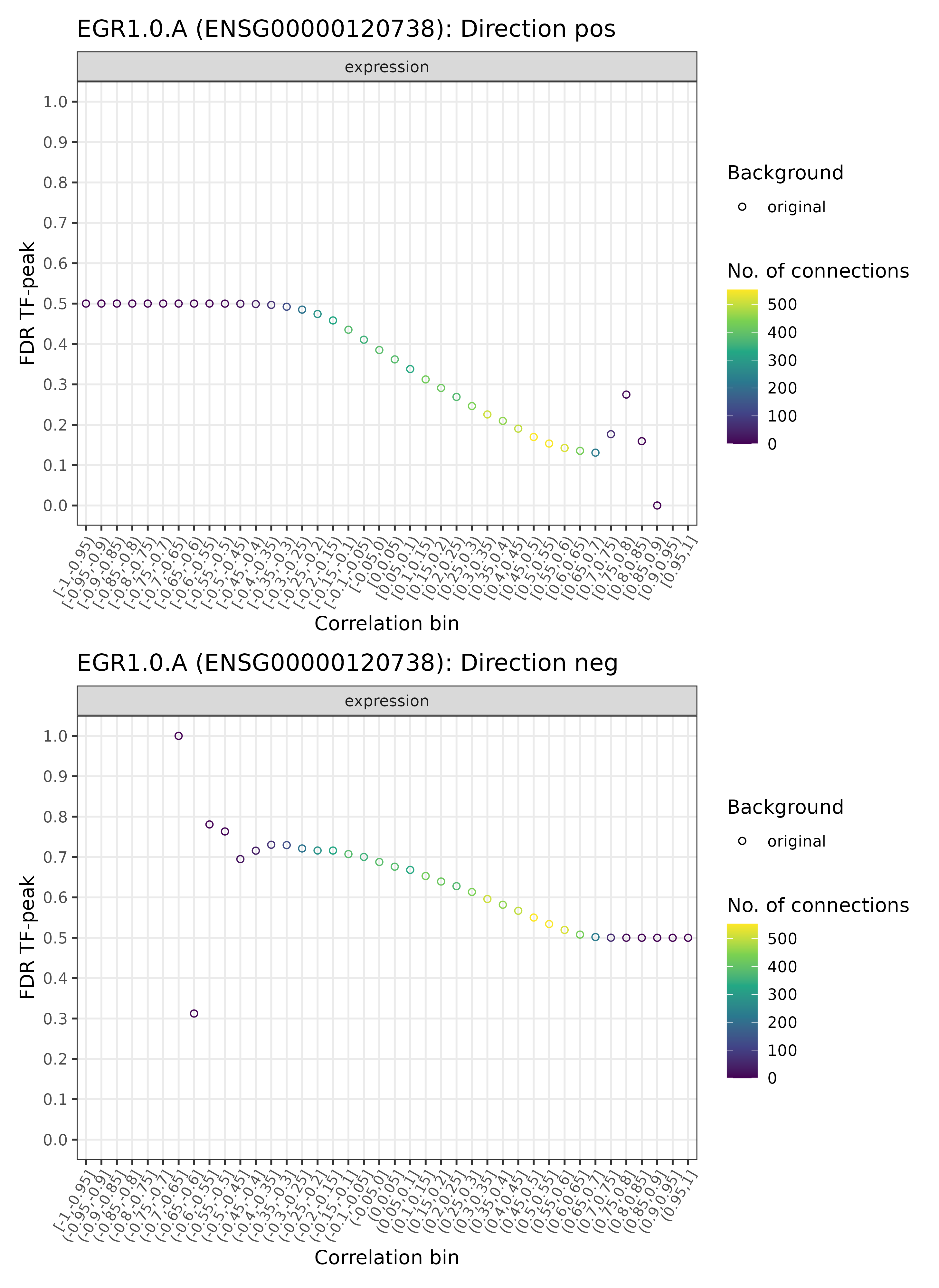
TF-enhancer diagnostic plots for EGR1.0.A (real)
## INFO [2023-08-16 17:38:32]
##  Plotting for Real data
## INFO [2023-08-16 17:38:32] Plotting FDR summary and curves for each TF
## INFO [2023-08-16 17:38:32]  Including a total of 65 TF. Preparing plots...
## INFO [2023-08-16 17:38:33]  Finished successfully. Execution time: 0.9 secs
## INFO [2023-08-16 17:38:33] Finished successfully. Execution time: 1 secs
We here picked an exemplary TF that appears on page 42 in the output
PDF as produced by the function. Remember that by setting
plotAsPDF = FALSE, one can plot specific pages directly to
the currently active graphics device instead of plotting all pages to a
PDF (the default). Here, we can see a quite typical case: the
TF-enhancer FDR for the various EGR1.0.A - enhancer pairs are
above 0.2 for the wide majority correlation bins in both directions
(that is, positive and negative), while a few bins for the positive
direction towards for more extreme correlation bins have a lower FDR
< 0.2 and one bin even with FDR < 0.1. The former indicate little
statistical signal and confidence, while the latter are those
connections we are looking for! Typically, however, only few connections
are in the more extreme bins, as indicated by the darker color (see the
legend). Here, correlation bin refers to the correlation of a particular
EGR1.0.A - enhancer pair that has been discretized accordingly
(i.e., a correlation of 0.07 would go into (0.05-0.10] correlation bin).
Usually, depending on the mode of action of a TF, none or either one of
the two directions may show a low FDR in particular areas of the plots,
often close to more extreme correlation bins, but rarely both. For a
better judgement and interpretation, we can also check how this looks
like for the background data:
GRN = plotDiagnosticPlots_TFPeaks(GRN, dataType = c("background"), plotAsPDF = FALSE,
    pages = c(42))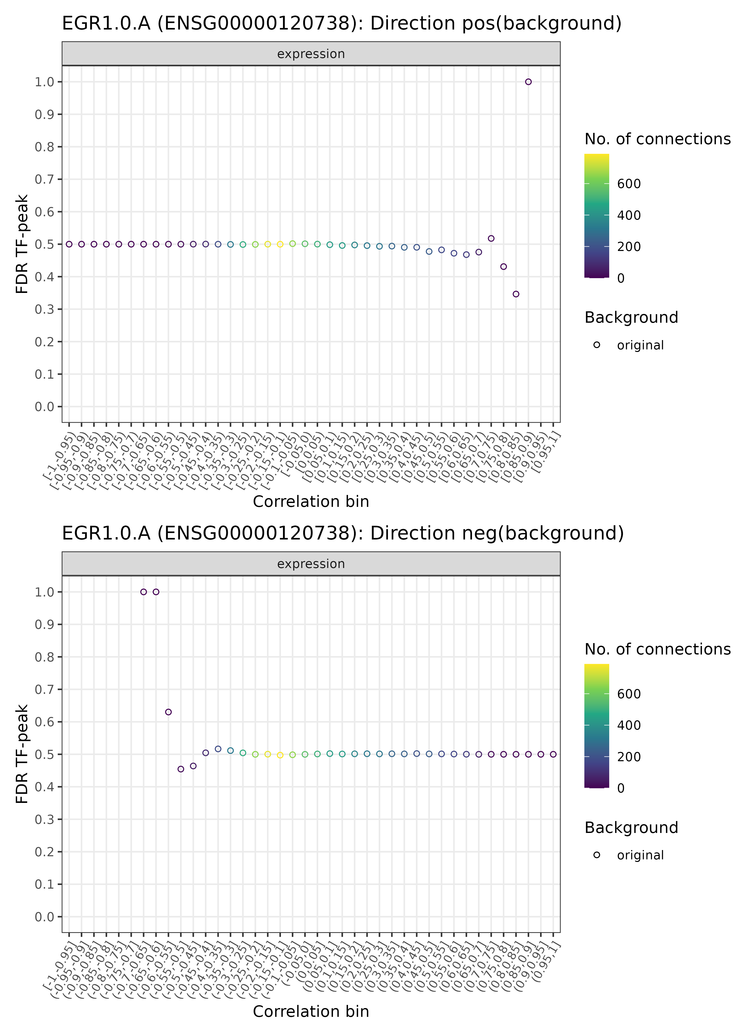
TF-enhancer diagnostic plots for EGR1.0.A (background)
## INFO [2023-08-16 17:38:36]
##  Plotting for Permuted data
## INFO [2023-08-16 17:38:36] Plotting FDR summary and curves for each TF
## INFO [2023-08-16 17:38:36]  Including a total of 65 TF. Preparing plots...
## INFO [2023-08-16 17:38:37]  Finished successfully. Execution time: 1 secs
## INFO [2023-08-16 17:38:37] Finished successfully. Execution time: 1 secs
Much fewer significant bins (one bin with FDR < 0.2), as expected.
In summary, a few positively correlated EGR1.0.A - enhancer
pairs (with a correlation of above 0.5 or so) are statistically
significant and may be retained for the final eGRN network
(if corresponding genes connecting to the respective enhancers are
found). As mentioned before, for more details, see also the Package
Details.
Run the AR classification and QC (optional)
Transcription factors (TFs) regulate many cellular processes and can
therefore serve as readouts of the signaling and regulatory state. Yet
for many TFs, the mode of action—repressing or activating transcription
of target genes—is unclear. In analogy to our diffTF approach
that we recently published to calculate differential TF activity,the
classification of TFs into putative transcriptional activators or
repressors can also be done from within the GRaNIE
framework in an identical fashion. This can be achieved with the
function AR_classification_wrapper().
Note that this step is fully optional and can be skipped. The
output of the function is not used for subsequent steps.. To
keep the memory footprint of the GRaNIE object low, we
recommend to keep the function parameter default
deleteIntermediateData = TRUE. Here, we specify to put all
plots within the directory plots. However, for reasons of
brevity, we do not actually run the code here.
GRN = AR_classification_wrapper(GRN, significanceThreshold_Wilcoxon = 0.05, outputFolder = "plots",
    plot_minNoTFBS_heatmap = 100, plotDiagnosticPlots = TRUE, forceRerun = TRUE)
The classification runs for both real and background data, as before.
The contents of these plots are identical to and uses in fact
practically the same code as our diffTF software, and we
therefore do not include them here. We refer to the following links for
more details as well as the Package Details
Vignette:
- The
official
diffTFpaper - In general, the ReadTheDocs
documentaion, and in particular this chapter. In
File {comparisonType}.diagnosticPlotsClassification1.pdf:, pages 1-4, the content of the filesTF_classification_stringencyThresholdsare explained in detail, while inFile {comparisonType}.diagnosticPlotsClassification2.pdf:, Page 20 - endthe contents of the filesTF_classification_summaryHeatmapandTF_classification_densityPlotsForegroundBackgroundare elaborated upon.
For more parameter details, see also the R help
(?AR_classification_wrapper).
Save GRaNIE object to disk (optional)
After steps that take up a bit of time, it may make sense to store
the GRaNIE object to disk in order to be able to restore it
at any time point. This can simply be done, for example, by saving it as
an rds file using the built-in function
saveRDS from R to save our GRaNIE object in a
compressed rds format.
You can then, at any time point, read it back into R with the following line:
GRN = readRDS(GRN_file_outputRDS)
Add enhancer-gene connections
Let’s add now the second type of connections, enhancer-genes, to
connect our enhancers to genes! This can be done via the function
addConnections_peak_gene(). This function has a few
parameters, and we only touch upon a few of them here. Most importantly,
the promoterRange specifies the neighborhood size,
which denotes the maximum neighborhood size in bp for enhancers (for
both upstream and downstream ) to find genes in vicinity and
associate/correlate genes with enhancers. While the default is 250,000
bp, we here set it to just 10,000 bp for computational reasons. Also, we
support the incorporation of TADs if available to replace the
default fixed neighborhood-based approach by a more flexible,
biologically-driven chromatin domain based approach. Here, we do not
have TADs available, so we set it to NULL. For more
parameter details, see the R help
(?addConnections_peak_gene).
GRN = addConnections_peak_gene(GRN, corMethod = "pearson", promoterRange = 10000,
    TADs = NULL, nCores = 1, plotDiagnosticPlots = FALSE, plotGeneTypes = list(c("all")),
    forceRerun = TRUE)
## INFO [2023-08-16 17:38:40]
## Real data
##
## INFO [2023-08-16 17:38:40] Calculate peak-gene correlations for neighborhood size 10000
## INFO [2023-08-16 17:38:40] Calculate peak gene overlaps...
## INFO [2023-08-16 17:38:40] Extend peaks based on user-defined extension size of 10000 up- and downstream.
## INFO [2023-08-16 17:38:41] Finished successfully. Execution time: 1.3 secs
## INFO [2023-08-16 17:38:42] Iterate through 41912 peak-gene combinations and calculate correlations using 1 cores. This may take a few minutes.
## INFO [2023-08-16 17:38:57] Finished execution using 1 cores. TOTAL RUNNING TIME: 15.5 secs
##
## INFO [2023-08-16 17:38:57] Finished with calculating correlations, creating final data frame and filter NA rows due to missing RNA-seq data
## INFO [2023-08-16 17:38:57] Initial number of rows: 41912
## INFO [2023-08-16 17:38:58] Finished. Final number of rows: 18902
## INFO [2023-08-16 17:38:58] Finished successfully. Execution time: 17.6 secs
## INFO [2023-08-16 17:38:58]
## Permuted data
##
## INFO [2023-08-16 17:38:58] Calculate random peak-gene correlations for neighborhood size 10000
## INFO [2023-08-16 17:38:58] Calculate peak gene overlaps...
## INFO [2023-08-16 17:38:58] Extend peaks based on user-defined extension size of 10000 up- and downstream.
## INFO [2023-08-16 17:38:58] Finished successfully. Execution time: 0.5 secs
## INFO [2023-08-16 17:38:58] Randomize gene-peak links by shuffling the peak IDs.
## INFO [2023-08-16 17:38:59] Iterate through 41912 peak-gene combinations and calculate correlations using 1 cores. This may take a few minutes.
## INFO [2023-08-16 17:39:11] Finished execution using 1 cores. TOTAL RUNNING TIME: 12.8 secs
##
## INFO [2023-08-16 17:39:11] Finished with calculating correlations, creating final data frame and filter NA rows due to missing RNA-seq data
## INFO [2023-08-16 17:39:11] Initial number of rows: 41912
## INFO [2023-08-16 17:39:12] Finished. Final number of rows: 18902
## INFO [2023-08-16 17:39:12] Finished successfully. Execution time: 13.9 secs
## INFO [2023-08-16 17:39:12] Finished successfully. Execution time: 31.6 secsWe see from the output that almost 38,000 enhancer-gene links have been identified that match our parameters. However, only around 16,351 actually had corresponding RNA-seq data available, while RNA-seq data was missing or has been filtered for the other. This is a rather typical case, as not all known and annotated genes are included in the RNA-seq data in the first place. Similar to before, the correlations have also been calculated for the background links (for details, see the Package Details).
Quality control 3: Diagnostic plots for enhancer-gene connections
Let’s now check some diagnostic plots for the enhancer-gene connections. In analogy to the TF-enhancer diagnostic plots that we encountered already before, we describe their interpretation and meaning in more detail in the Package Details!
The following plot summarizes many key QC measures we implemented:
GRN = plotDiagnosticPlots_peakGene(GRN, gene.types = list(c("protein_coding", "lincRNA")),
    plotAsPDF = FALSE, pages = 1)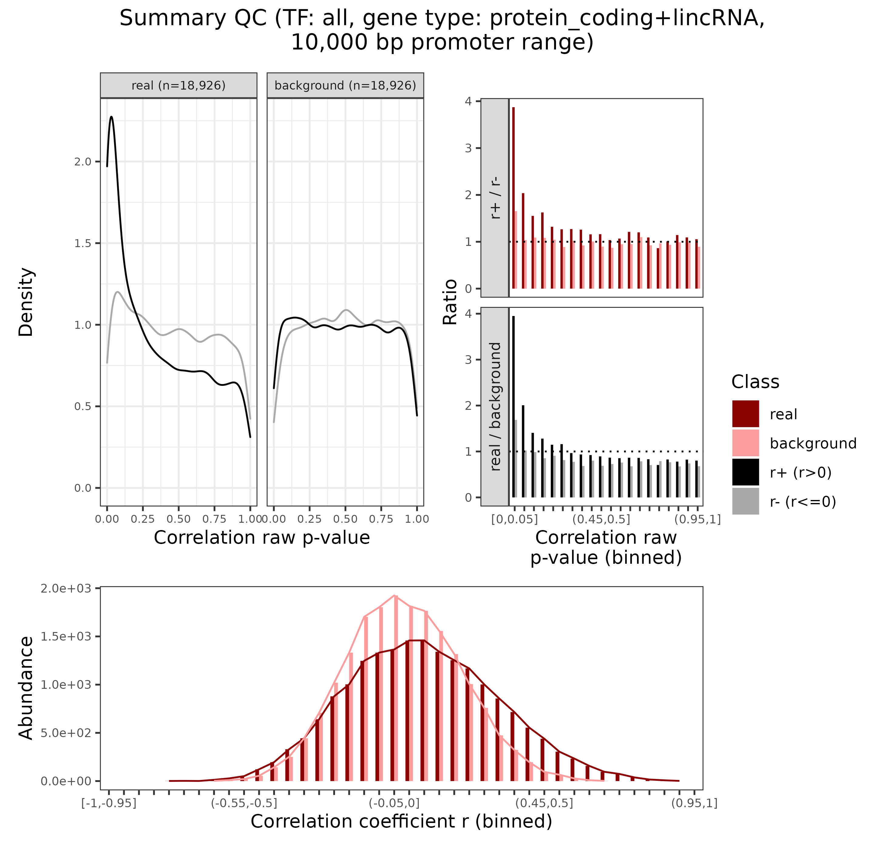
Enhancer-gene diagnostic plots
## INFO [2023-08-16 17:39:12] Plotting diagnostic plots for peak-gene correlations
## INFO [2023-08-16 17:39:12]  Gene type protein_coding+lincRNA
## INFO [2023-08-16 17:39:14]  Finished successfully. Execution time: 1.8 secs
## INFO [2023-08-16 17:39:14] Finished successfully. Execution time: 1.8 secs
Without explaining the details here, we can see from mainly the upper left plot that the enhancer-gene connections show a good signal to noise ratio in the context of our framework and assumptions indeed! For more details, see also here
Combine TF-enhancer and enhancer-gene connections and filter
Now that we added both TF-enhancers and enhancer-gene links to our
GRaNIE object, we are ready to filter and combine them. So
far, they are stored separately in the object for various reasons (see
the Introductory Vignette for details), but ultimately, we aim for
combining them to derive TF-enhancer-gene connections. To do so, we can
simply run the filterGRNAndConnectGenes() function and
filter the individual TF-enhancer and enhancer-gene links to our liking.
The function has many more arguments, and we only specify a few in the
example below. As before, we get a GRaNIE object back that
now contains the merged and filtered TF-enhancer-gene connections that
we can later extract. Some of the filters apply to the TF-enhancer
links, some of them to the enhancer-gene links, the parameter name is
intended to indicate that.
GRN = filterGRNAndConnectGenes(GRN, TF_peak.fdr.threshold = 0.2, peak_gene.fdr.threshold = 0.2,
    peak_gene.fdr.method = "BH", gene.types = c("protein_coding", "lincRNA"), allowMissingTFs = FALSE,
    allowMissingGenes = FALSE, forceRerun = TRUE)
## Warning in .checkAndLogWarningsAndErrors(NULL, message, isWarning = TRUE): To avoid object inconsistencies and unexpected/non-reproducible results, the graph slot in the object has been reset. For all network-related functions as well as eGRN visualization, rerun the method build_eGRN_graph and all other network-related ans enrichment functions to update to the new set of filtered connections.
## This warning may or may not be ignored. Carefully check its significance and whether it may affect the results.## INFO [2023-08-16 17:39:15] Filter GRN network
## INFO [2023-08-16 17:39:15]
##
## Real data
## INFO [2023-08-16 17:39:15] Inital number of rows left before all filtering steps: 23096
## INFO [2023-08-16 17:39:15] Filter network and retain only rows with TF-peak connections with an FDR < 0.2
## INFO [2023-08-16 17:39:15] Number of TF-peak rows before filtering TFs: 23096
## INFO [2023-08-16 17:39:15] Number of TF-peak rows after filtering TFs: 4907
## INFO [2023-08-16 17:39:15] 2. Filter peak-gene connections
## INFO [2023-08-16 17:39:15] Filter genes by gene type, keep only the following gene types: protein_coding, lincRNA
## INFO [2023-08-16 17:39:15] Number of peak-gene rows before filtering by gene type: 18926
## INFO [2023-08-16 17:39:15] Number of peak-gene rows after filtering by gene type: 18830
## INFO [2023-08-16 17:39:15] 3. Merging TF-peak with peak-gene connections and filter the combined table...
## INFO [2023-08-16 17:39:15] Inital number of rows left before filtering steps: 5966
## INFO [2023-08-16 17:39:15] Filter TF-TF self-loops
## INFO [2023-08-16 17:39:15] Number of rows before filtering genes: 5966
## INFO [2023-08-16 17:39:15] Number of rows after filtering genes: 4021
## INFO [2023-08-16 17:39:15] Filter rows with missing ENSEMBL IDs
## INFO [2023-08-16 17:39:15] Number of rows before filtering: 4021
## INFO [2023-08-16 17:39:15] Number of rows after filtering: 4021
## INFO [2023-08-16 17:39:16] Filter network and retain only rows with peak_gene.r in the following interval: (0 - 1]
## INFO [2023-08-16 17:39:16] Number of rows before filtering: 4021
## INFO [2023-08-16 17:39:16] Number of rows after filtering: 2372
## INFO [2023-08-16 17:39:16] Calculate FDR based on remaining rows, filter network and retain only rows with peak-gene connections with an FDR < 0.2
## INFO [2023-08-16 17:39:16] Number of rows before filtering genes (including/excluding NA): 2372/2372
## INFO [2023-08-16 17:39:16] Number of rows after filtering genes (including/excluding NA): 626/626
## INFO [2023-08-16 17:39:16] Final number of rows left after all filtering steps: 626
## INFO [2023-08-16 17:39:16]
##
## Permuted data
## INFO [2023-08-16 17:39:16] Inital number of rows left before all filtering steps: 54
## INFO [2023-08-16 17:39:16] Filter network and retain only rows with TF-peak connections with an FDR < 0.2
## INFO [2023-08-16 17:39:16] Number of TF-peak rows before filtering TFs: 54
## INFO [2023-08-16 17:39:16] Number of TF-peak rows after filtering TFs: 31
## INFO [2023-08-16 17:39:16] 2. Filter peak-gene connections
## INFO [2023-08-16 17:39:16] Filter genes by gene type, keep only the following gene types: protein_coding, lincRNA
## INFO [2023-08-16 17:39:16] Number of peak-gene rows before filtering by gene type: 18926
## INFO [2023-08-16 17:39:16] Number of peak-gene rows after filtering by gene type: 18830
## INFO [2023-08-16 17:39:16] 3. Merging TF-peak with peak-gene connections and filter the combined table...
## INFO [2023-08-16 17:39:16] Inital number of rows left before filtering steps: 33
## INFO [2023-08-16 17:39:16] Filter TF-TF self-loops
## INFO [2023-08-16 17:39:16] Number of rows before filtering genes: 33
## INFO [2023-08-16 17:39:16] Number of rows after filtering genes: 13
## INFO [2023-08-16 17:39:16] Filter rows with missing ENSEMBL IDs
## INFO [2023-08-16 17:39:16] Number of rows before filtering: 13
## INFO [2023-08-16 17:39:16] Number of rows after filtering: 13
## INFO [2023-08-16 17:39:16] Filter network and retain only rows with peak_gene.r in the following interval: (0 - 1]
## INFO [2023-08-16 17:39:16] Number of rows before filtering: 13
## INFO [2023-08-16 17:39:16] Number of rows after filtering: 6
## INFO [2023-08-16 17:39:16] Calculate FDR based on remaining rows, filter network and retain only rows with peak-gene connections with an FDR < 0.2
## INFO [2023-08-16 17:39:16] Number of rows before filtering genes (including/excluding NA): 6/6
## INFO [2023-08-16 17:39:16] Number of rows after filtering genes (including/excluding NA): 0/0
## INFO [2023-08-16 17:39:16] Final number of rows left after all filtering steps: 0
## WARN [2023-08-16 17:39:16] To avoid object inconsistencies and unexpected/non-reproducible results, the graph slot in the object has been reset. For all network-related functions as well as eGRN visualization, rerun the method build_eGRN_graph and all other network-related ans enrichment functions to update to the new set of filtered connections.
## This warning may or may not be ignored. Carefully check its significance and whether it may affect the results.
##
## INFO [2023-08-16 17:39:16] Finished successfully. Execution time: 1 secsThe output shows the number of links before and after applying a particular filter that has been set for both real and background eGRN. As expected and reassuringly, almost no connections remain for the background eGRN, while the real one consists of around 2500 connections.
Importantly, this filtered set of connections is now also
saved in the GRN object and the basis for most if not all
downstream functions that the package offers and that this vignettes
mentions and that we explore now! It is important to keep
that in mind: Re-running the filterGRNAndConnectGenes()
method overwrites the all.filtered slot in the
GRN object, and all downstream functions have to be re-run
as well.
For more parameter details, see the R help
(?filterGRNAndConnectGenes).
Add TF-gene correlations (optional)
Optionally, we can also include extra columns about the correlation
of TF and genes directly. So far, only TF-enhancers and enhancer-genes
have been correlated, but not directly TFs and genes with each other.
Based on a filtered set of TF-enhancer-gene connections, the function
add_TF_gene_correlation() calculates the TF-gene
correlation for each connection from the filtered set for which the TF
is not missing.
GRN = add_TF_gene_correlation(GRN, corMethod = "pearson", nCores = 1, forceRerun = TRUE)## INFO [2023-08-16 17:39:17] Calculate correlations for TF and genes from the filtered set of connections
## INFO [2023-08-16 17:39:17] Real data
## INFO [2023-08-16 17:39:17] Iterate through 582 TF-gene combinations and (if possible) calculate correlations using 1 cores. This may take a few minutes.
## INFO [2023-08-16 17:39:17] Finished execution using 1 cores. TOTAL RUNNING TIME: 0.4 secs
##
## INFO [2023-08-16 17:39:17] Done. Construct the final table, this may result in an increased number of TF-gene pairs due to different TF names linked to the same Ensembl ID.
## INFO [2023-08-16 17:39:17] Permuted data
## INFO [2023-08-16 17:39:17] Nothing to do, skip.
## INFO [2023-08-16 17:39:17] Finished successfully. Execution time: 0.6 secsAs can be seen from the output, the Pearson correlation for all
TF-gene pairs has been calculated. The newly calculated information is
added to the object, and can be retrieved as shown in the next section.
For more details, see the R help
(?add_TF_gene_correlation).
Time to save our object again!
GRN = deleteIntermediateData(GRN)
saveRDS(GRN, GRN_file_outputRDS)
Retrieve filtered connections
After combining TF-peaks and peak-genes to a tripartite GRN, we are
now ready to retrieve the filtered connections, along with adding
various additional metadata (optional). This can be done with the helper
function getGRNConnections() that retrieves the filtered
eGRN as a data frame from a GRaNIE object.
Here, we specify all.filtered, as we want to retrieve all
filtered connections (i.e., the eGRN). For more parameter
details and an explanation of the columns from the returned
data frame, see the R help
(?getGRNConnections).
Here, for example, we add various additional information to the
resulting data frame: TF-gene correlations, and gene metadata. We could
also add TF and peak metadata as well as the results from running the
variancePartition package, but this is not done here and we
leave this as an exercise to the reader!
Note that the first time, we assign a different variable to the
return of the function (i.e., GRN_connections.all and NOT
GRN as before). Importantly, we have to select a new
variable as we would otherwise overwrite our GRN object
altogether! All get functions from the GRaNIE
package return an element from within the object and NOT the object
itself, so please keep that in mind and always check what the functions
returns before running it. You can simply do so in the R help
(?getGRNConnections).
GRN_connections.all = getGRNConnections(GRN, type = "all.filtered", include_TF_gene_correlations = TRUE,
    include_geneMetadata = TRUE)

GRN_connections.all
## # A tibble: 626 × 25
## TF.ID TF.name TF.EN…¹ peak.ID TF_pe…² TF_pe…³ TF_pe…⁴ TF_pe…⁵ TF_pe…⁶ peak_…⁷
## <fct> <fct> <fct> <fct> <fct> <dbl> <dbl> <fct> <fct> <int>
## 1 BATF… BATF3.… ENSG00… chr7:1… [0.65,… 0.684 0.185 pos expres… 4874
## 2 E2F6… E2F6.0… ENSG00… chr15:… [0.55,… 0.550 0.156 pos expres… 145
## 3 E2F6… E2F6.0… ENSG00… chr6:4… [0.5,0… 0.514 0.175 pos expres… 154
## 4 E2F6… E2F6.0… ENSG00… chr3:4… [0.5,0… 0.539 0.175 pos expres… 0
## 5 E2F6… E2F6.0… ENSG00… chr1:6… [0.5,0… 0.539 0.175 pos expres… 0
## 6 E2F6… E2F6.0… ENSG00… chr17:… [0.45,… 0.494 0.191 pos expres… 6011
## 7 E2F6… E2F6.0… ENSG00… chr7:1… [0.55,… 0.585 0.156 pos expres… 0
## 8 E2F6… E2F6.0… ENSG00… chr6:1… [0.5,0… 0.501 0.175 pos expres… 3990
## 9 E2F6… E2F6.0… ENSG00… chr1:6… [0.65,… 0.663 0.166 pos expres… 1004
## 10 E2F6… E2F6.0… ENSG00… chr6:4… [0.5,0… 0.528 0.175 pos expres… 9262
## # … with 616 more rows, 15 more variables: peak_gene.r <dbl>,
## # peak_gene.p_raw <dbl>, peak_gene.p_adj <dbl>, gene.ENSEMBL <chr>,
## # gene.name <fct>, gene.type <fct>, gene.mean <dbl>, gene.median <dbl>,
## # gene.CV <dbl>, gene.chr <fct>, gene.start <int>, gene.end <int>,
## # gene.strand <fct>, TF_gene.r <dbl>, TF_gene.p_raw <dbl>, and abbreviated
## # variable names ¹TF.ENSEMBL, ²TF_peak.r_bin, ³TF_peak.r, ⁴TF_peak.fdr,
## # ⁵TF_peak.fdr_direction, ⁶TF_peak.connectionType, ⁷peak_gene.distanceThe table contains many columns, and the prefix of each column name
indicates the part of the eGRN network that the column
refers to (e.g., TFs, TF-enhancers, enhancers, enhancer-genes or genes,
or TF-gene if the function add_TF_gene_correlation() has
been run before). As mentioned above, see the R help
(?getGRNConnections) for an explanation of the
columns. Data are stored in a format that minimizes the memory
footprint (e.g., each character column is stored as a factor). This
table can now be used for any downstream analysis, as it is just a
normal data frame.
Generate a connection summary for filtered connections
It is often useful to get a grasp of the general connectivity of a
network and the number of connections that survive the filtering. This
makes it possible to make an informed decision about which FDR to choose
for TF-enhancer and enhancer-gene links, depending on how many links are
retained and how many connections are needed for downstream analysis. To
facilitate this and automate it, we offer the convenience function
generateStatsSummary() that in essence iterates over
different combinations of filtering parameters and calls the function
filterGRNAndConnectGenes() once for each of them, and then
records various connectivity statistics, and finally plots it by calling
the function plot_stats_connectionSummary(). Note that
running this function may take a while. Afterwards, we can graphically
summarize this result in either a heatmap or a boxplot. For more
parameter details, see the R help (?generateStatsSummary
and ?plot_stats_connectionSummary).
GRN = generateStatsSummary(GRN, TF_peak.fdr = c(0.05, 0.1, 0.2), TF_peak.connectionTypes = "all",
    peak_gene.fdr = c(0.1, 0.2), peak_gene.r_range = c(0, 1), allowMissingGenes = c(FALSE,
        TRUE), allowMissingTFs = c(FALSE), gene.types = c("protein_coding", "lincRNA"),
    forceRerun = TRUE)


GRN = plot_stats_connectionSummary(GRN, type = "heatmap", plotAsPDF = FALSE, pages = 3)
GRN = plot_stats_connectionSummary(GRN, type = "boxplot", plotAsPDF = FALSE, pages = 1)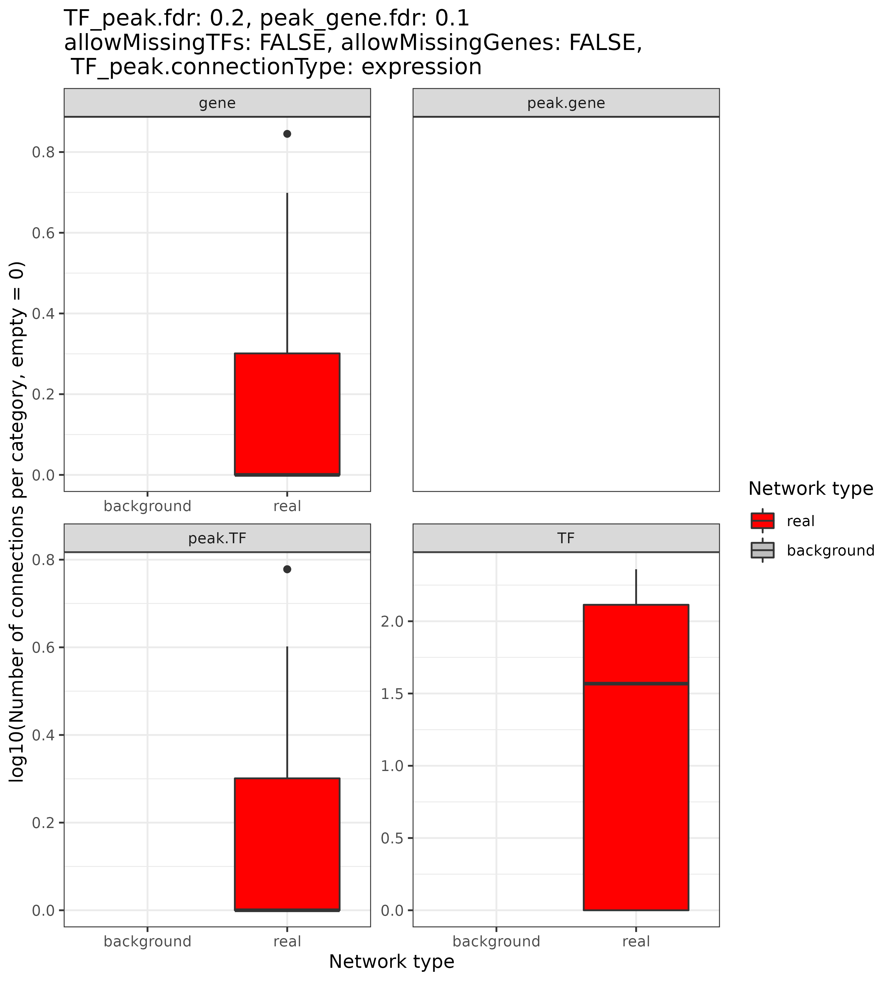
## INFO [2023-08-16 17:39:19] Generating summary. This may take a while...
## INFO [2023-08-16 17:39:19]
## Real data...
##
## INFO [2023-08-16 17:39:19] Calculate network stats for TF-peak FDR of 0.05
## INFO [2023-08-16 17:39:22] Calculate network stats for TF-peak FDR of 0.1
## INFO [2023-08-16 17:39:26] Calculate network stats for TF-peak FDR of 0.2
## INFO [2023-08-16 17:39:29]
## Permuted data...
##
## INFO [2023-08-16 17:39:29] Calculate network stats for TF-peak FDR of 0.05
## INFO [2023-08-16 17:39:33] Calculate network stats for TF-peak FDR of 0.1
## INFO [2023-08-16 17:39:36] Calculate network stats for TF-peak FDR of 0.2
## INFO [2023-08-16 17:39:39] Finished successfully. Execution time: 20.2 secs
## INFO [2023-08-16 17:39:39] Plotting connection summary
## INFO [2023-08-16 17:39:40]  Finished successfully. Execution time: 0.9 secs
## INFO [2023-08-16 17:39:40] Finished successfully. Execution time: 0.9 secs
## INFO [2023-08-16 17:39:40] Plotting diagnostic plots for network connections
## INFO [2023-08-16 17:39:41]  Finished successfully. Execution time: 0.8 secs
## INFO [2023-08-16 17:39:41] Finished successfully. Execution time: 0.8 secs
Here, the output is less informative and just tells us about the current progress and parameter it iterates over. We can now check the two new PDF files that have been created!
Let’s start with a connection summary in form of a heatmap! There are
3 heatmap classes, one for TFs, enhancers (labeled peaks) and genes,
respectively. All of them compare the number of distinct TFs, enhancers,
and genes that end up in the final eGRN in dependence of
how stringently the connections are filtered (i.e., different FDR
thresholds for both TF-enhancers and enhancer-genes). In addition, the
same is repeated for the background eGRN, which enables you to judge the
connectivity of the real eGRN as compared to what you can
expect with random data!
For TFs, we see that the numbers are generally very small because we just run the analysis with few TFs. For the background eGRN, none or almost none connections survive the filtering. You should see much bigger differences for full TF data and not just a few selected ones.
As the output plots show, alternatively, we can also represent the
connectivity in form of a boxplot, which shows the connectivity for each
node or connection type (i.e. TFs, enhancers, and genes, while enhancers
are split between TF-enhancer and enhancer-gene depending on whether
they connect with TFs or genes, respectively), and compares this again
to the random version of the eGRN. The PDF contains many
pages, and iterates over different FDR stringency thresholds. We here
show two example pages:
Not all parameter combinations (such as FDR stringencies) result in
connections! Sometimes, there is no eGRN as no connections
survived the filtering.
For more details, see also the Package Details!
Construct the eGRN graph
For all network-related and visualization-related functions, we need to build a graph out of the filtered connections. For this, we provide a helper function that stores the graph-structure in the object, and it can be invoked as follows:
GRN = build_eGRN_graph(GRN, forceRerun = TRUE)## INFO [2023-08-16 17:39:42] Building TF-peak-gene graph...
## INFO [2023-08-16 17:39:42] Graph summary:
## INFO [2023-08-16 17:39:42] Nodes (vertices): 816
## INFO [2023-08-16 17:39:42] Edges: 1013
## INFO [2023-08-16 17:39:42] Done. Graphs are saved in GRN@graph
## INFO [2023-08-16 17:39:42] Building TF-gene graph...
## INFO [2023-08-16 17:39:42] Graph summary:
## INFO [2023-08-16 17:39:42] Nodes (vertices): 411
## INFO [2023-08-16 17:39:42] Edges: 582
## INFO [2023-08-16 17:39:42] Done. Graphs are saved in GRN@graph
## INFO [2023-08-16 17:39:42] Finished successfully. Execution time: 0.2 secsAs you can see, some details about the TF-peak-gene and TF-gene are
shown as output. As mentioned before, the graph is constructed based on
the filtered connections as calculated and stored by
filterGRNAndConnectGenes(). Importantly, the graph is reset
whenever the function filterGRNAndConnectGenes() is called
either directly or indirectly via
generateStatsSummary().
Visualize the eGRN
The GRaNIE package also offers a function to visualize a
filtered eGRN network! It is very easy to invoke, but
provides many options to customize the output and the way the graph is
drawn. We recommend to explore the options in the R help
(?getGRNConnections), and here just run the default
visualization. By default, eGRNs with 500 edges or less can
be plotted with the default options, which prevents from plotting large
number of networks that cannot be visualized nicely anyway. However,
this can be customized to also draw larger networks (see the parameter
maxEdgesToPlot and the notes below) and is being utilized
here:
GRN = visualizeGRN(GRN, plotAsPDF = FALSE, maxEdgesToPlot = 1000)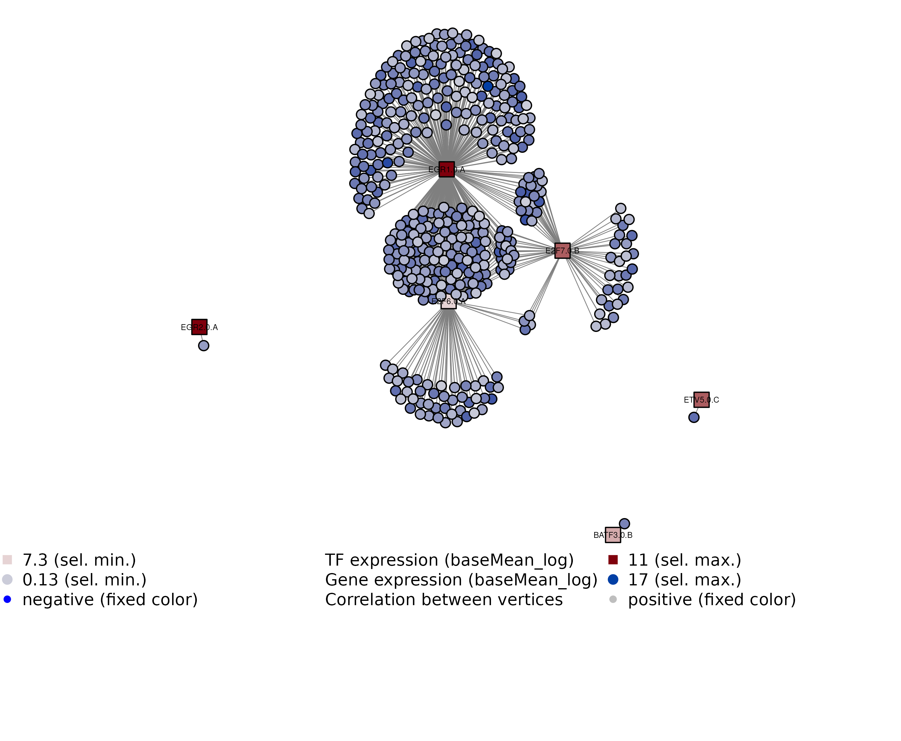
eGRN example visualization
## INFO [2023-08-16 17:39:43] Number of edges for the TF-gene eGRN graph: 582
## INFO [2023-08-16 17:39:43] Plotting many connections may need a lot of time and memory
## INFO [2023-08-16 17:39:43] Plotting GRN network
## INFO [2023-08-16 17:39:44]  Finished successfully. Execution time: 0.9 secs
We can see some highly connected TFs and that they actually seem to co-regulate some shared genes. The selection of TFs here for this toy dataset was based on highly connected TFs across all TF, though, so for a larger list of TFs, expect to see some TFs being not connected much or at all, though.
Visualizing a larger network is naturally more challenging. If your
visualization does not work or it does not look clear or nice enough,
check out the Package
Details for recommendations. We now also provide the function
filterConnectionsForPlotting() to filter a eGRN
just for visualization purposes. This reduces the number of nodes and
edges to plot and gives the user ultimate flexibility of what to
visualize. For example, you can filter the network to just visualize the
part of the network that is connected to a specific set of TFs (i.e,
their regulons). The filter criteria can be flexibly defined via
dplyr style syntax as either one or multiple arguments, see
the example that follows:
GRN = filterConnectionsForPlotting(GRN, plotAll = FALSE, TF.ID == "E2F7.0.B" | stringr::str_starts(TF.ID,
    "ETV"))
GRN = visualizeGRN(GRN, plotAsPDF = FALSE)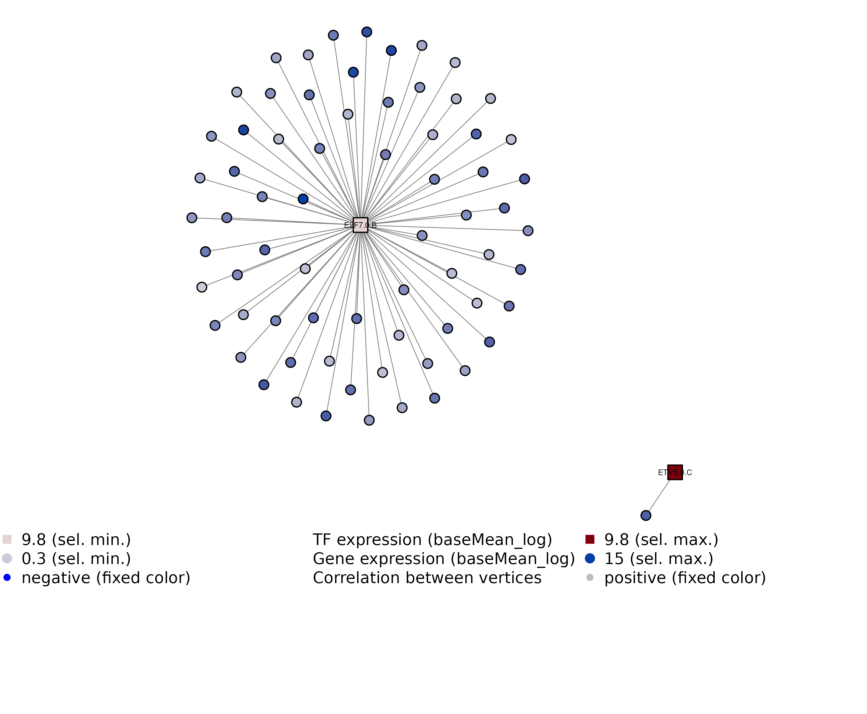
eGRN example visualization with extra filtering
## INFO [2023-08-16 17:39:45]  Filter connections for GRN visualization
## INFO [2023-08-16 17:39:45]  Keep connections for a total of 73 connections
## INFO [2023-08-16 17:39:45] Number of edges for the TF-gene eGRN graph: 70
## INFO [2023-08-16 17:39:45] Plotting GRN network
## INFO [2023-08-16 17:39:45]  Finished successfully. Execution time: 0.2 secs
Network and enrichment analyses for filtered connections
Lastly, our framework also supports various types of network and
enrichment analyses that are fully integrated into the package. We offer
these for the full filtered eGRN network as a whole (as
produced by running the function filterGRNAndConnectGenes()
before) as well as an enrichment per community.
First, a proper graph (network) structure can be build with the
function build_eGRN_graph(), which all network and
enrichment functions use subsequently.
For both the general and the community statistics and enrichment, the package can:
- calculate and plot general structure and connectivity statistics for
a filtered
eGRN(functionplotGeneralGraphStats()) and per community (functionscalculateCommunitiesStats()andplotCommunitiesStats()) , - ontology enrichment and visualization for genes for the full network
(functions
calculateGeneralEnrichment()andplotGeneralEnrichment()) as well as per community (functionscalculateCommunitiesEnrichment()andplotCommunitiesEnrichment())
All functions can be called individually, adjusted flexibly and the
data is stored in the GRaNIE object for ultimate
flexibility. In the near future, we plan to expand this set of
functionality to additional enrichment analyses such as other databases
(specific diseases pathways etc), so stay tuned!
calculateCommunitiesStats()
For the purpose of this vignette, let’s run an enrichment
analysis using GO. here, we run it with only
GO Biological Process (GO_BP), while the other
GO ontologies are also available (i.e.,
GO Molecular Function, abbreviated GO_MF in
the plots). We also support other, more specialized enrichment analyses
(KEGG, Disease Ontology, and
Reactome). Lastly, users can select an arbitrary
combination of all supported ontologies for ultimate flexibility! More
are coming soon, stay tuned!
For user convenience, all aforementioned functions can be called at
once via a designated wrapper function
performAllNetworkAnalyses(). Many results are produces by
this convenience function, and we here show only a few of them. The
function is highly customizable, all or almost all of the available
parameters from the individual functions (see above) are also available
in this wrapper function, see the R help
(?performAllNetworkAnalyses) for details. In order to
invoke it and save all results to several PDF files using the default
options, for example, you could simply type this:
GRN = performAllNetworkAnalyses(GRN, ontology = c("GO_BP"), outputFolder = ".", forceRerun = TRUE)As this functions needs a few minutes, for the purpose of the vignette, we do not include the output of this function here. Let’s, however, go through all the functions that this wrapper executes so we have a better understanding of what is actually being done. We will also plot some of the results!
First, we have to create a network representation out of the filtered
connections, and there are a few options for how the network structure
should look like. We here keep the default options and refer to the R
help for details (?build_eGRN_graph).
General network statistics
Let’s, however, check some of the results that are produced! Let’s start with checking some general network statistics for the full network. From the various graphs that are produced, we here select only 2 of them for demonstration purposes. First we can check the vertex distribution and gene types for the overall network to get an idea of how the network looks like. Second, we can investigate the most important TFs and genes for the network for both the TF-enhancer-gene as well as TF-gene network. Here, we here show the results for the TF-gene network only:
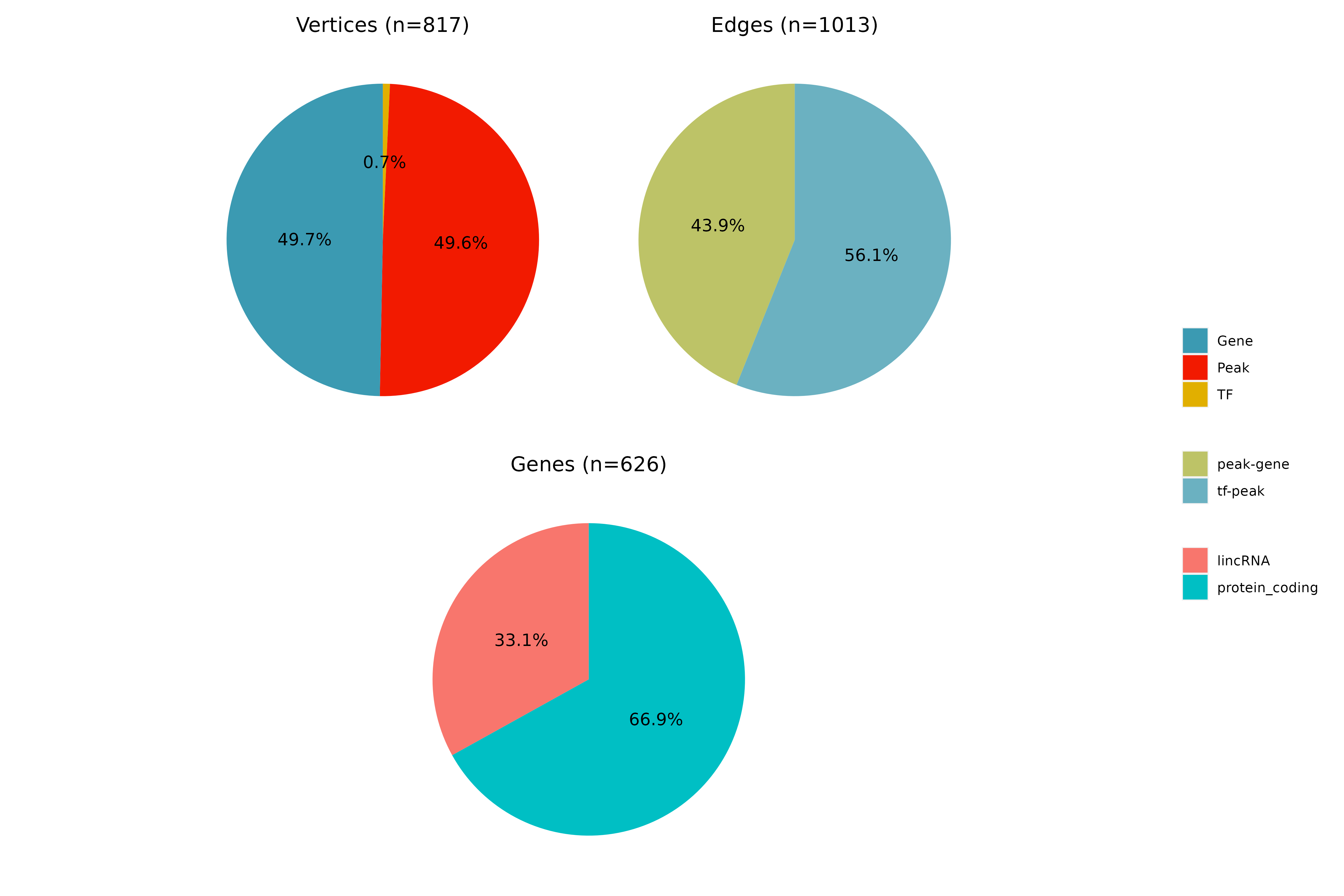
General network statistics for the filtered network
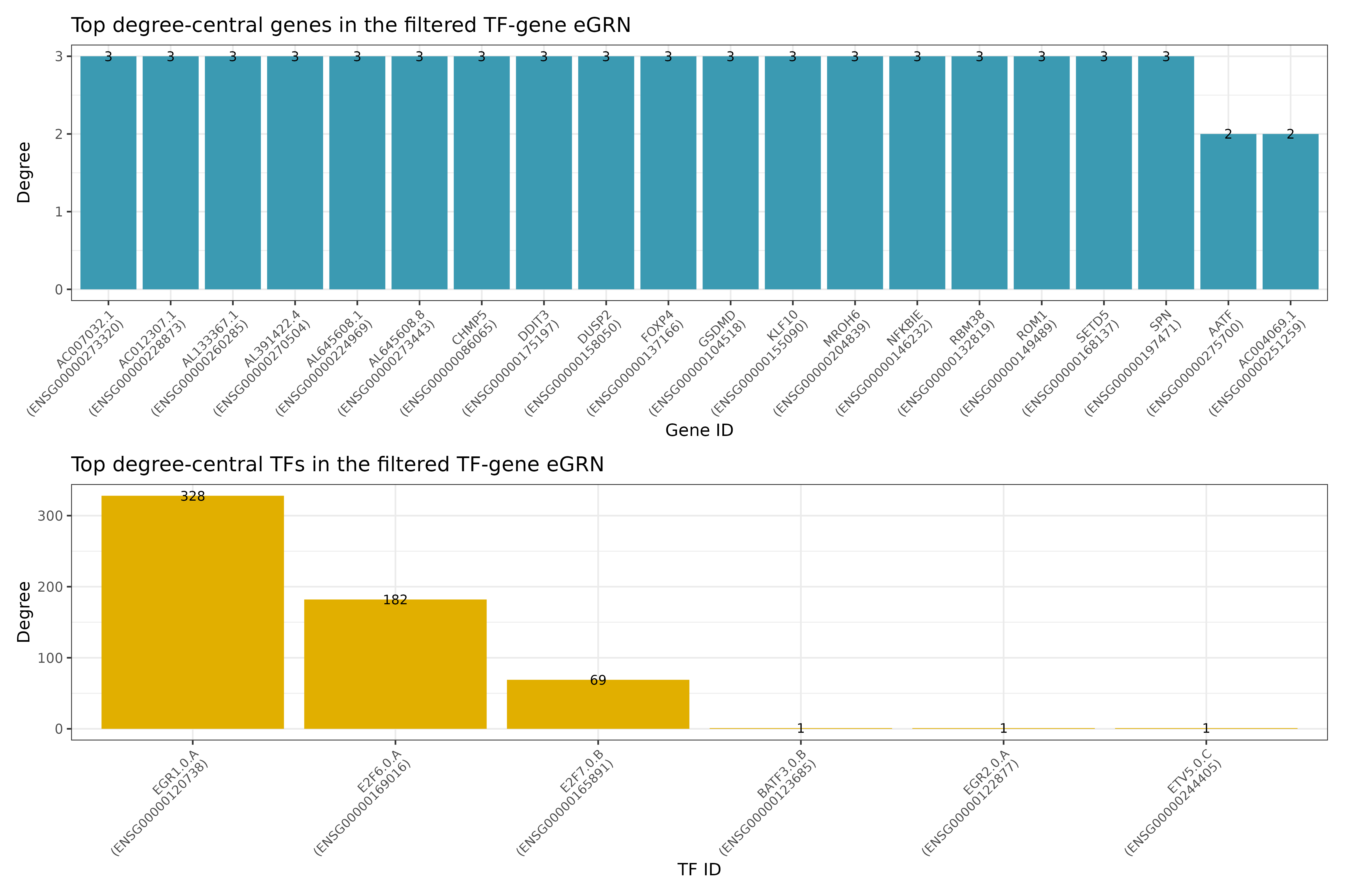
General network statistics for the filtered network
## INFO [2023-08-16 17:39:46] Plotting directly
## INFO [2023-08-16 17:39:48]  Finished successfully. Execution time: 1.9 secs
First, we see the vertex degree of TF and genes, respectively: We can also use algorithms for measuring the influence of a node in a network (centrality). Here, we show the results for both TFs and genes for two different measures of centrality, eigenvector centrality and centrality based on node degree:
General network enrichment
Now that we have our eGRN network, we can do various
enrichment analyses. Let’s start with the most obvious one: Enrichment
for the whole network. Again, we are not executing the function here for
reasons of time, but you should do so of course when learning how to use
the package!
We can now plot the enrichment for the full graph. In analogy to all
the other plot functions, a PDF with all enrichment results
is produced with the default setting, but by setting
plotAsPDF to FALSE, we can also plot selected
results / pages directly to the currently active graphics device. In
this case here, as we select only one ontology, there is only one
page:
GRN = plotGeneralEnrichment(GRN, plotAsPDF = FALSE, pages = 1)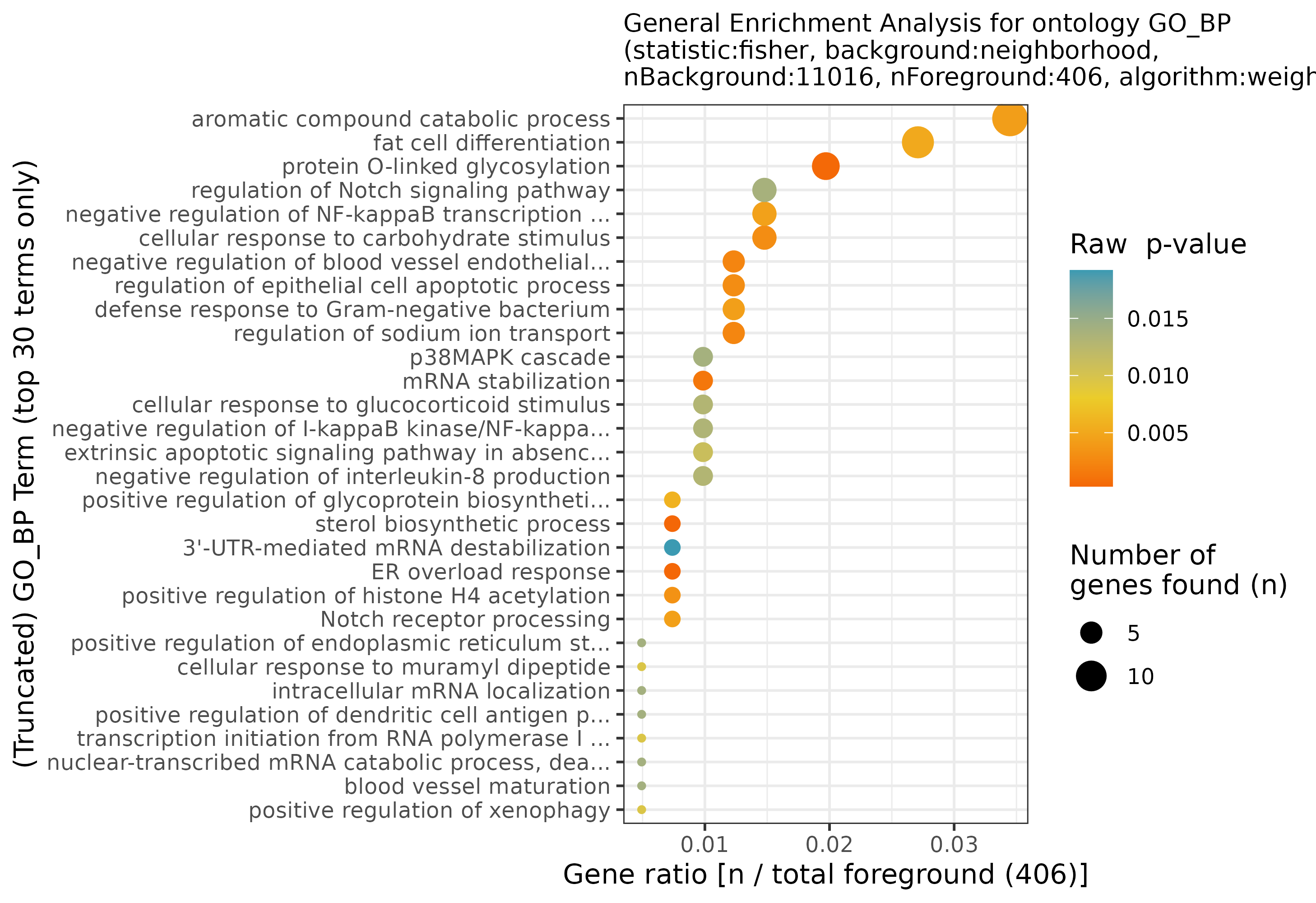
General network enrichment for the filtered network
## INFO [2023-08-16 17:39:52] Plotting directly
## INFO [2023-08-16 17:39:52] Found the following ontology results for plotting: GO_BP,GO_MF
## INFO [2023-08-16 17:39:52] Plotting for the following user-selected ontologies: GO_BP,GO_MF
## INFO [2023-08-16 17:39:52]  Ontology GO_BP
## INFO [2023-08-16 17:39:52]  Ontology GO_MF
## INFO [2023-08-16 17:39:52]  Finished successfully. Execution time: 0.3 secs
We can see that overall, cell cycle is the term with the most number of genes, and while it does not have the highest significance among all terms, it is still significant. Most of the other terms are more specialized, and point towards altered regulation of various epigenetic signaling alterations. The biological plausibility of them and how to continue after is now your challenge!
Community network statistics and enrichment
Now, let’s check whether we can identify communities within the whole network, along with community-specific enrichments.
## INFO [2023-08-16 17:39:53] Calculating communities for clustering type louvain...
## INFO [2023-08-16 17:39:53] Community summary for all 6 communities (Number of nodes per community, sorted by community size):
## INFO [2023-08-16 17:39:53]  Community 1: 174 nodes
## INFO [2023-08-16 17:39:53]  Community 5: 161 nodes
## INFO [2023-08-16 17:39:53]  Community 4: 70 nodes
## INFO [2023-08-16 17:39:53]  Community 2: 2 nodes
## INFO [2023-08-16 17:39:53]  Community 3: 2 nodes
## INFO [2023-08-16 17:39:53]  Community 6: 2 nodes
## INFO [2023-08-16 17:39:53]  Finished successfully. Execution time: 0.1 secs
## INFO [2023-08-16 17:39:54] Running enrichment analysis for all 6 communities. This may take a while...
## INFO [2023-08-16 17:39:54]  Community 1
## INFO [2023-08-16 17:39:54] Data already exists in object or the specified file already exists. Set forceRerun = TRUE to regenerate and overwrite.
## INFO [2023-08-16 17:39:54]  Community 2
## INFO [2023-08-16 17:39:54] Data already exists in object or the specified file already exists. Set forceRerun = TRUE to regenerate and overwrite.
## INFO [2023-08-16 17:39:54]  Community 3
## INFO [2023-08-16 17:39:54] Data already exists in object or the specified file already exists. Set forceRerun = TRUE to regenerate and overwrite.
## INFO [2023-08-16 17:39:54]  Community 4
## INFO [2023-08-16 17:39:54] Data already exists in object or the specified file already exists. Set forceRerun = TRUE to regenerate and overwrite.
## INFO [2023-08-16 17:39:54]  Community 5
## INFO [2023-08-16 17:39:54] Data already exists in object or the specified file already exists. Set forceRerun = TRUE to regenerate and overwrite.
## INFO [2023-08-16 17:39:54]  Community 6
## INFO [2023-08-16 17:39:54] Data already exists in object or the specified file already exists. Set forceRerun = TRUE to regenerate and overwrite.
## INFO [2023-08-16 17:39:54]  Finished successfully. Execution time: 0.8 secs
These functions may take a while, as enrichment is calculated for each community. Once finished, we are ready to plot the results! First, let’s start with some general community statistics:
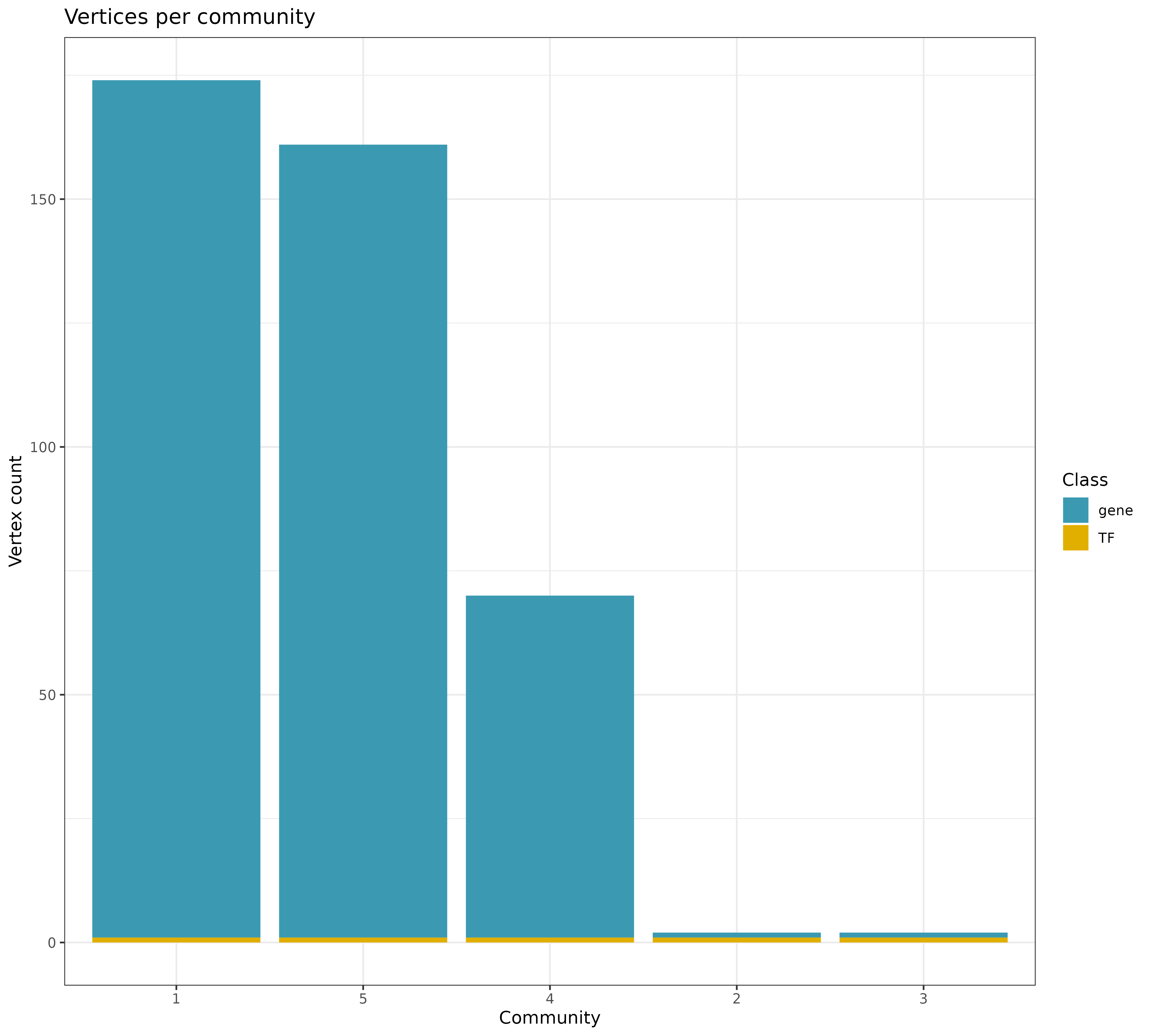
General statistics for the communities from the filtered network
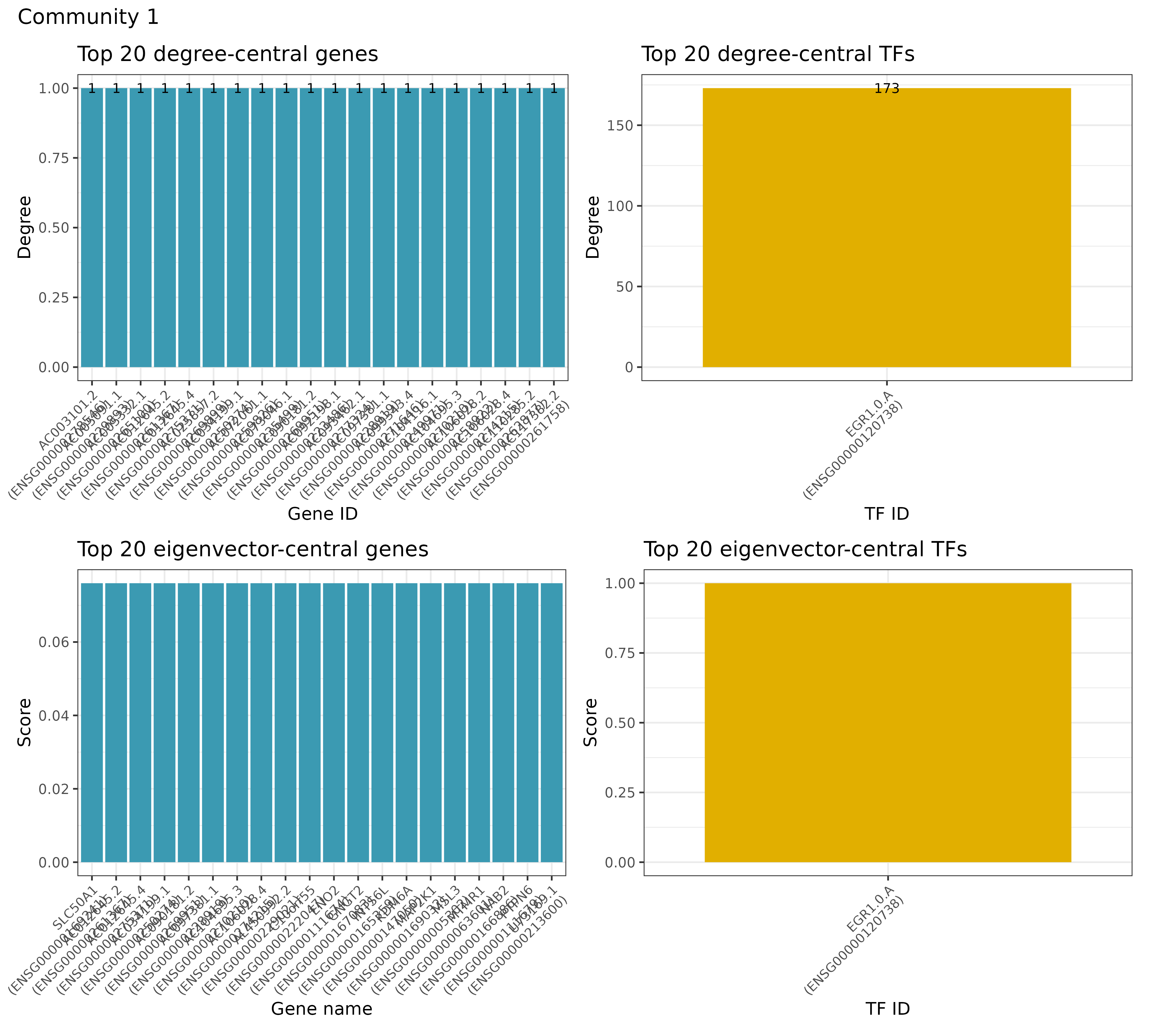
General statistics for the communities from the filtered network
## INFO [2023-08-16 17:39:54] Plotting directly
## INFO [2023-08-16 17:39:57]  Finished successfully. Execution time: 2.6 secs
First, we see an overview across all communities and their network sizes, and whether the links belong to a TF or gene. Second, for a selected community, we summarize which genes and TFs are most relevant for this particular community. Because the example data is rather minimal, this looks very unspectacular here: Only one TF appears in the list, and all connected genes have the same node degree also. For real datasets, this will look more interesting and diverse.
Next, let’s plot the community-specific enrichment:
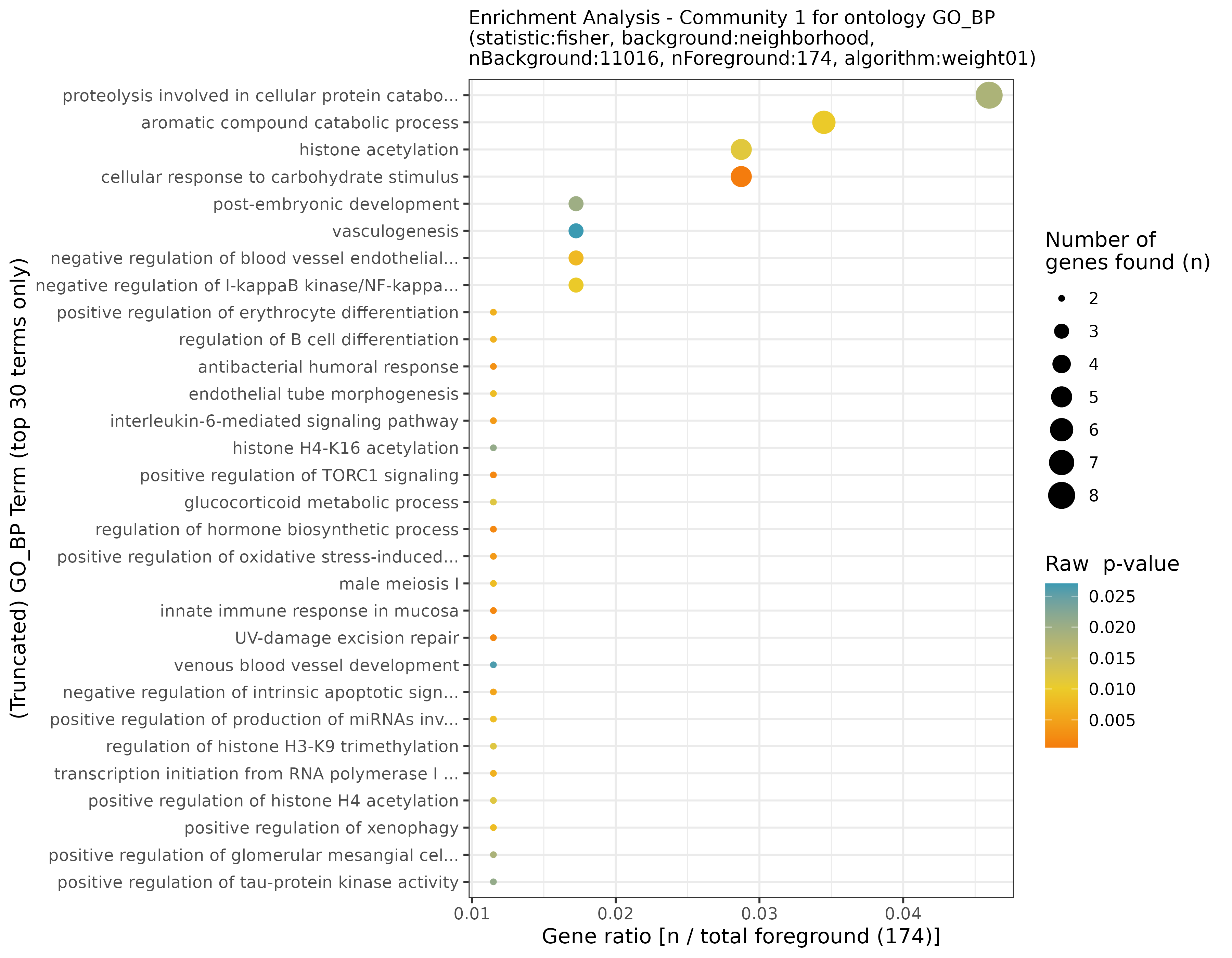
Community enrichment for 3 different communities
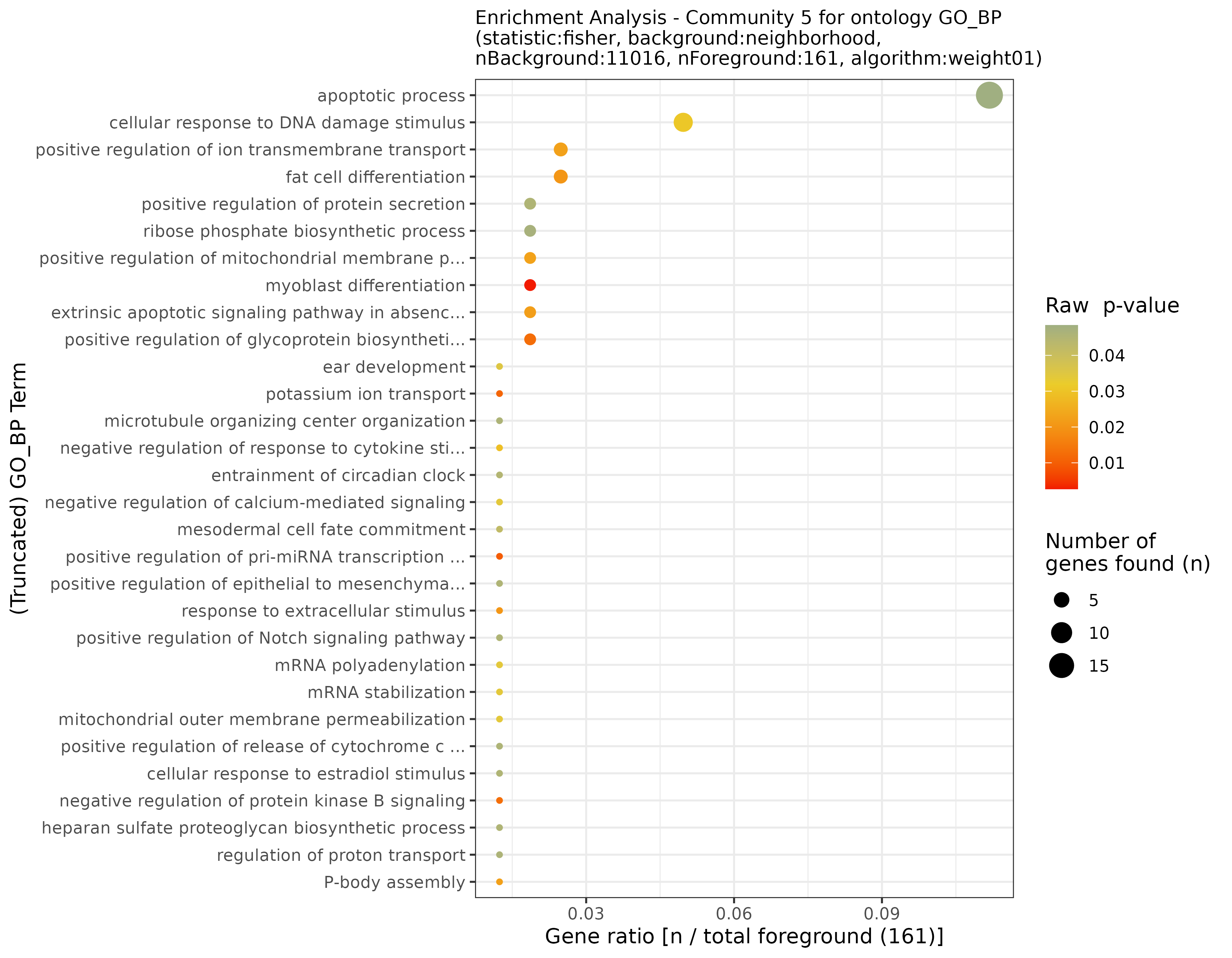
Community enrichment for 3 different communities
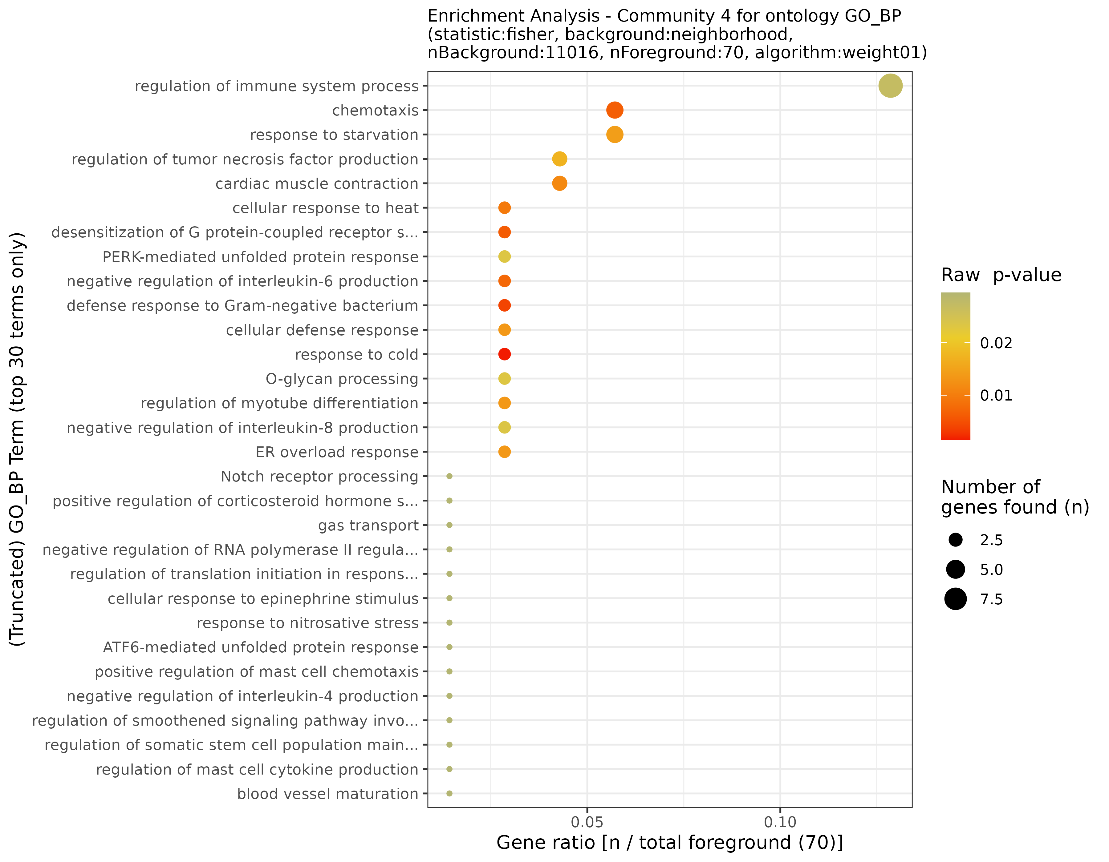
Community enrichment for 3 different communities
## INFO [2023-08-16 17:40:00] Including terms only if overlap is at least 2 genes.
## INFO [2023-08-16 17:40:00]  Plotting the enrichment for the following communities: 1,5,4,2,3,6
## INFO [2023-08-16 17:40:00] Plotting directly
## INFO [2023-08-16 17:40:00]  Plotting results for ontology GO_BP
## INFO [2023-08-16 17:40:02]  Plotting results for ontology GO_MF
## INFO [2023-08-16 17:40:03]  Finished successfully. Execution time: 3 secs
We also provide an overview across the whole network and all communities that lists all the enriched terms that appear in at least one enrichment analysis, so a direct comparison of the specificity and commonalities across communities and between the general network and any community is facilitated. This also shows that some terms, here more than with a full dataset, are only identified as being enriched for the full network but not within any of the communities individually. We offer this function for all terms as well as only the top 10 enriched terms per community, and we here show only the filtered version due to reasons of brevity:
GRN = plotCommunitiesEnrichment(GRN, plotAsPDF = FALSE, pages = c(5))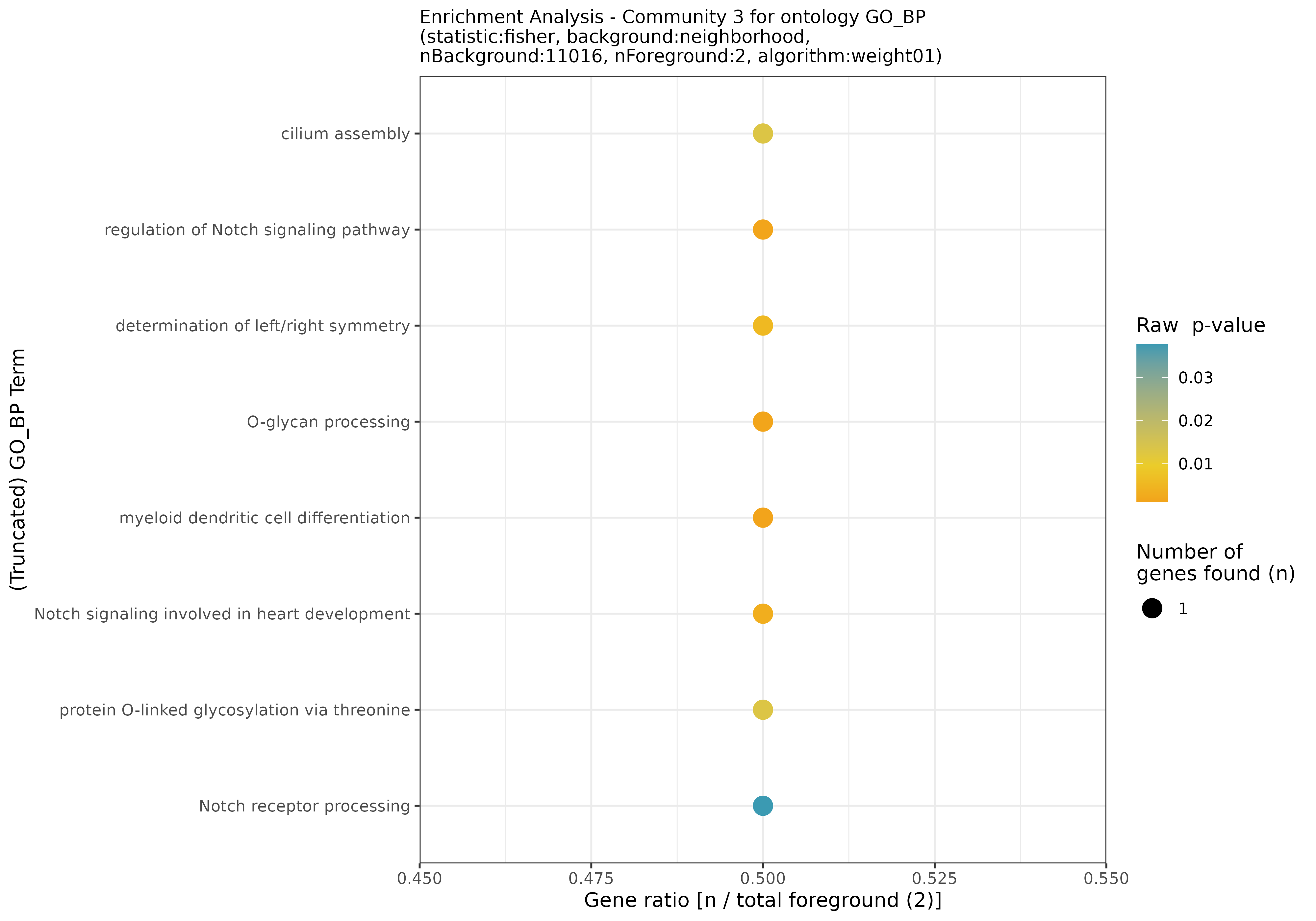
Summary of the community enrichment
## INFO [2023-08-16 17:40:06] Including terms only if overlap is at least 2 genes.
## INFO [2023-08-16 17:40:06]  Plotting the enrichment for the following communities: 1,5,4,2,3,6
## INFO [2023-08-16 17:40:06] Plotting directly
## INFO [2023-08-16 17:40:06]  Plotting results for ontology GO_BP
## INFO [2023-08-16 17:40:06]  Plotting results for ontology GO_MF
## INFO [2023-08-16 17:40:07]  Finished successfully. Execution time: 1.2 secs
TF enrichment analyses
In analogy to community enrichment, we can also calculate enrichment
based on TFs via their target genes they are connected to. Running a TF
enrichment analyses is straight forward, with the parameter
n we can control the number of TFs to run the enrichment
for - the function runs the enrichment for the top connected TFs. Thus,
n=3 equals running the enrichment for the top 3 connected
TFs. Here, we show the results for one of the TFs, EGR1.0.A, as
well as a summary across all top 3 connected TFs, in analogy the results
for the community enrichment.
Let’s first calculate the TF enrichment.This may take a while. We omit the output here.
Now, we can plot it, similar to the enrichment results before:
GRN = plotTFEnrichment(GRN, plotAsPDF = FALSE, n = 3, pages = c(1))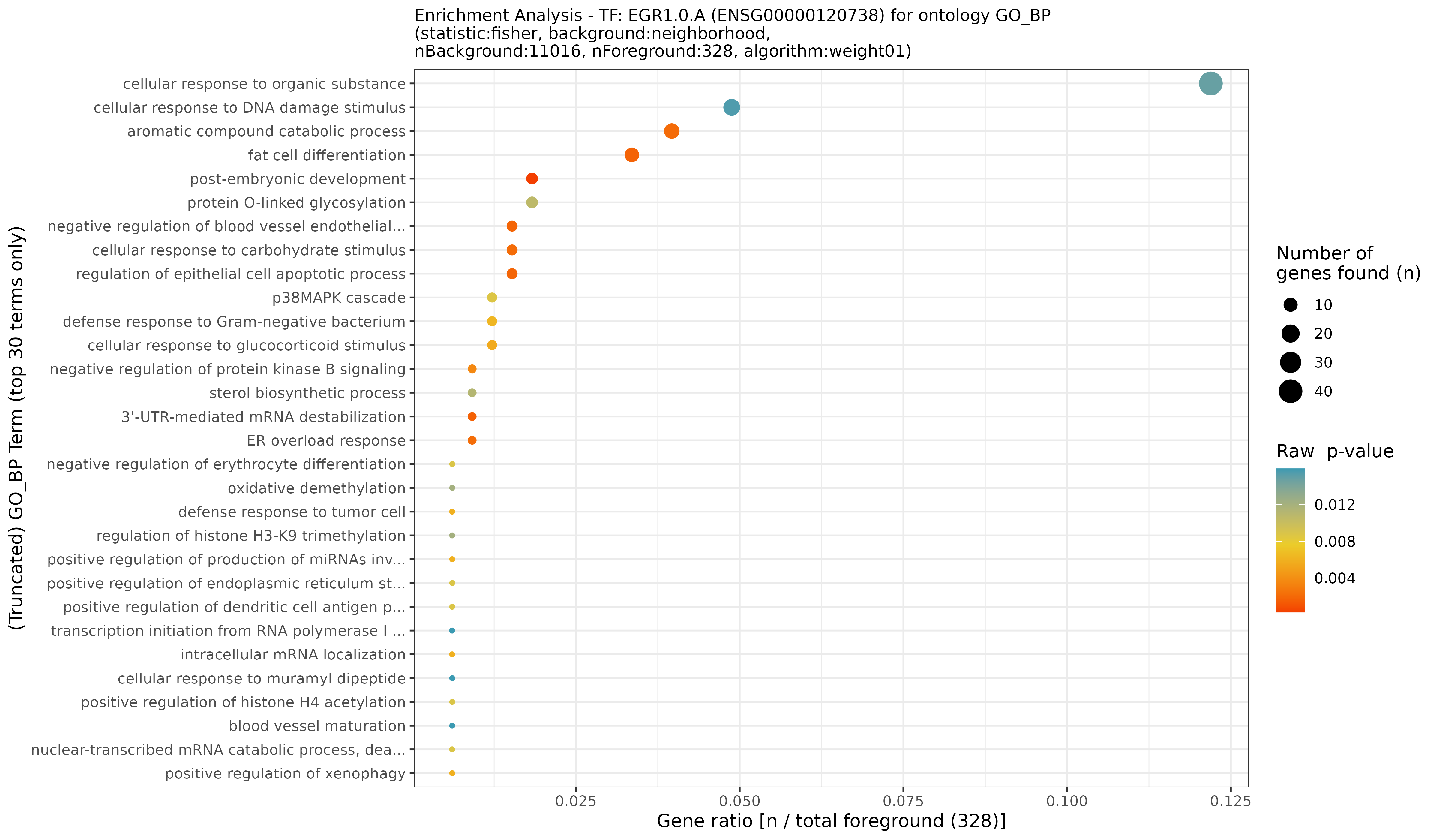
Enrichment summary for EGR1.0.A
## INFO [2023-08-16 17:40:09] n = 3 equals finding the top 3 degree-central TFs in the network
## INFO [2023-08-16 17:40:09]  Finished successfully. Execution time: 0.1 secs
## INFO [2023-08-16 17:40:09] Plotting directly
## INFO [2023-08-16 17:40:09]  Plotting results for ontology GO_BP
## INFO [2023-08-16 17:40:09]   TF EGR1.0.A (ENSG00000120738)
## INFO [2023-08-16 17:40:09]  Plotting results for ontology GO_MF
## INFO [2023-08-16 17:40:10]  Finished successfully. Execution time: 1.1 secs
GRN = plotTFEnrichment(GRN, plotAsPDF = FALSE, n = 3, pages = c(5))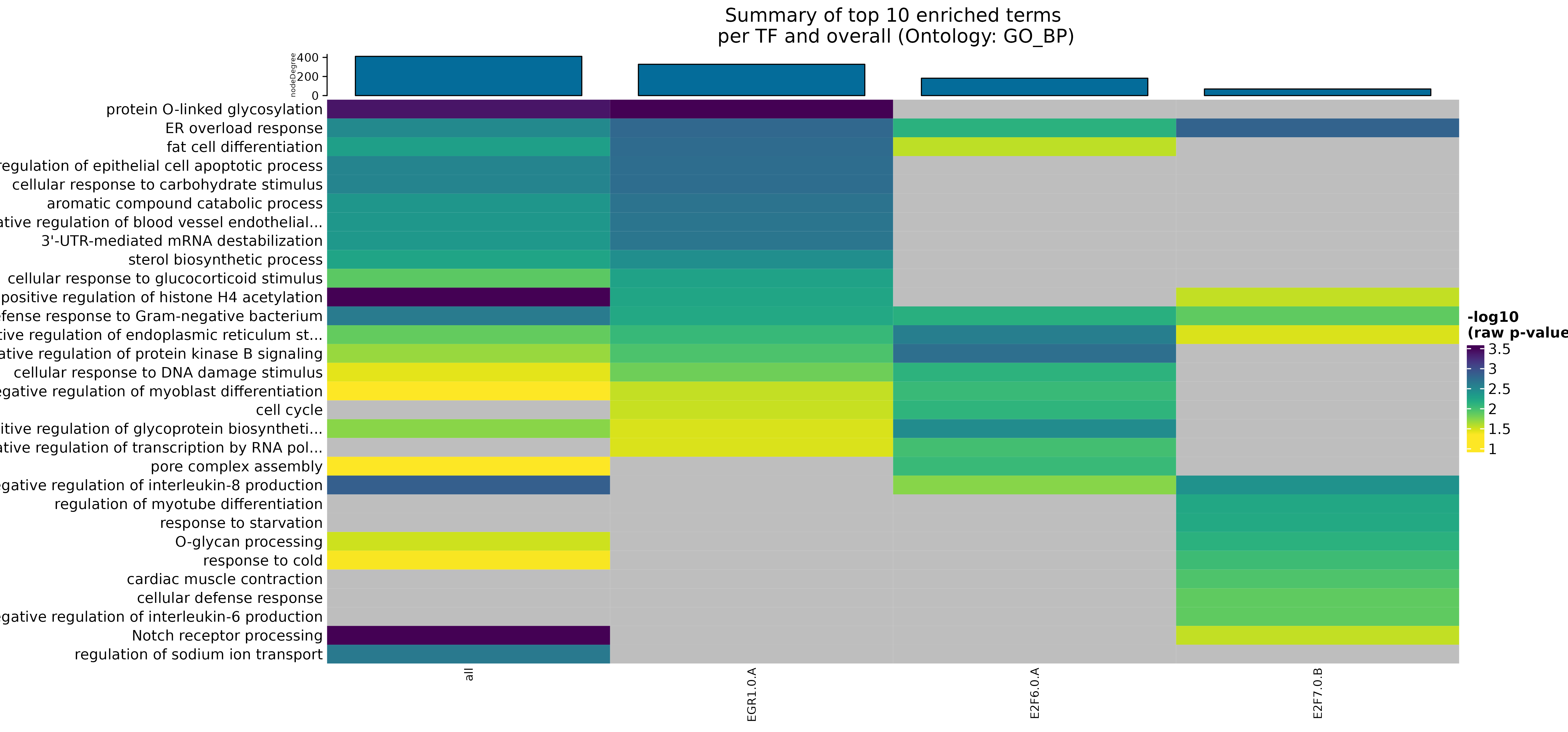
Enrichment summary for selected TFs and the whole eGRN network
## INFO [2023-08-16 17:40:11] n = 3 equals finding the top 3 degree-central TFs in the network
## INFO [2023-08-16 17:40:11]  Finished successfully. Execution time: 0 secs
## INFO [2023-08-16 17:40:11] Plotting directly
## INFO [2023-08-16 17:40:11]  Plotting results for ontology GO_BP
## INFO [2023-08-16 17:40:11]   Including 30 terms in the reduced summary heatmap and 4 columns
## INFO [2023-08-16 17:40:14]  Plotting results for ontology GO_MF
## INFO [2023-08-16 17:40:14]  Finished successfully. Execution time: 3.3 secs
Wrapping up
We are now finished with the main workflow, all that is left to do is
to save our GRaNIE object to disk so we can load it at a
later time point without having to repeat the analysis. We recommend to
run the convenience function deleteIntermediateData()
beforehand that aims to reduce its size by deleting some intermediate
data that may still be stored within the object. For more parameter
details, see the R help (?deleteIntermediateData). Finally,
as we did already in the middle of the workflow, we save the object
finally in rds format.
GRN = deleteIntermediateData(GRN)
saveRDS(GRN, GRN_file_outputRDS)
How to continue?
From here on, possibilities are endless, and you can further
investigate patterns and trends in the data! We hope that the
GRaNIE package is useful for your research and encourage
you to contact us if you have any question or feature request!
Session Info
## R version 4.2.1 (2022-06-23)
## Platform: x86_64-pc-linux-gnu (64-bit)
## Running under: Ubuntu 20.04.5 LTS
##
## Matrix products: default
## BLAS:   /usr/lib/x86_64-linux-gnu/blas/libblas.so.3.9.0
## LAPACK: /usr/lib/x86_64-linux-gnu/lapack/liblapack.so.3.9.0
##
## locale:
##  [1] LC_CTYPE=en_US.UTF-8       LC_NUMERIC=C
##  [3] LC_TIME=en_GB.UTF-8        LC_COLLATE=en_US.UTF-8
##  [5] LC_MONETARY=en_GB.UTF-8    LC_MESSAGES=en_US.UTF-8
##  [7] LC_PAPER=en_GB.UTF-8       LC_NAME=C
##  [9] LC_ADDRESS=C               LC_TELEPHONE=C
## [11] LC_MEASUREMENT=en_GB.UTF-8 LC_IDENTIFICATION=C
##
## attached base packages:
## [1] stats4    stats     graphics  grDevices utils     datasets  methods
## [8] base
##
## other attached packages:
## [1] GenomeInfoDb_1.35.15 IRanges_2.30.1       S4Vectors_0.34.0
## [4] BiocGenerics_0.42.0  GRaNIE_1.5.2         readr_2.1.2
## [7] knitr_1.40           BiocStyle_2.24.0
##
## loaded via a namespace (and not attached):
##   [1] backports_1.4.1             circlize_0.4.15
##   [3] BiocFileCache_2.4.0         systemfonts_1.0.4
##   [5] igraph_1.3.4                plyr_1.8.7
##   [7] lazyeval_0.2.2              BiocParallel_1.30.3
##   [9] ggplot2_3.3.6               digest_0.6.29
##  [11] foreach_1.5.2               ensembldb_2.20.2
##  [13] htmltools_0.5.3             GO.db_3.15.0
##  [15] magick_2.7.3                viridis_0.6.2
##  [17] fansi_1.0.3                 magrittr_2.0.3
##  [19] checkmate_2.1.0             memoise_2.0.1
##  [21] cluster_2.1.4               doParallel_1.0.17
##  [23] tzdb_0.3.0                  ComplexHeatmap_2.12.1
##  [25] Biostrings_2.64.1           matrixStats_0.62.0
##  [27] vroom_1.5.7                 pkgdown_2.0.6
##  [29] prettyunits_1.1.1           colorspace_2.0-3
##  [31] blob_1.2.3                  rappdirs_0.3.3
##  [33] textshaping_0.3.6           xfun_0.33
##  [35] dplyr_1.1.0                 crayon_1.5.1
##  [37] RCurl_1.98-1.8              jsonlite_1.8.0
##  [39] graph_1.74.0                iterators_1.0.14
##  [41] glue_1.6.2                  gtable_0.3.1
##  [43] zlibbioc_1.42.0             XVector_0.36.0
##  [45] GetoptLong_1.0.5            DelayedArray_0.22.0
##  [47] shape_1.4.6                 SparseM_1.81
##  [49] scales_1.2.1                futile.options_1.0.1
##  [51] DBI_1.1.3                   Rcpp_1.0.9
##  [53] viridisLite_0.4.1           progress_1.2.2
##  [55] clue_0.3-61                 bit_4.0.4
##  [57] httr_1.4.4                  RColorBrewer_1.1-3
##  [59] ellipsis_0.3.2              pkgconfig_2.0.3
##  [61] XML_3.99-0.10               farver_2.1.1
##  [63] sass_0.4.2                  dbplyr_2.2.1
##  [65] utf8_1.2.2                  tidyselect_1.2.0
##  [67] labeling_0.4.2              rlang_1.0.6
##  [69] reshape2_1.4.4              AnnotationDbi_1.58.0
##  [71] munsell_0.5.0               tools_4.2.1
##  [73] cachem_1.0.6                cli_3.4.0
##  [75] generics_0.1.3              RSQLite_2.2.17
##  [77] evaluate_0.16               stringr_1.5.0
##  [79] fastmap_1.1.0               yaml_2.3.5
##  [81] ragg_1.2.2                  bit64_4.0.5
##  [83] fs_1.5.2                    purrr_0.3.4
##  [85] KEGGREST_1.36.3             AnnotationFilter_1.20.0
##  [87] formatR_1.12                xml2_1.3.3
##  [89] biomaRt_2.52.0              compiler_4.2.1
##  [91] rstudioapi_0.14             filelock_1.0.2
##  [93] curl_4.3.2                  png_0.1-7
##  [95] tibble_3.1.8                bslib_0.4.0
##  [97] stringi_1.7.8               highr_0.9
##  [99] futile.logger_1.4.3         GenomicFeatures_1.48.3
## [101] desc_1.4.2                  forcats_0.5.2
## [103] lattice_0.20-45             ProtGenerics_1.28.0
## [105] Matrix_1.5-1                vctrs_0.5.2
## [107] pillar_1.8.1                lifecycle_1.0.3
## [109] BiocManager_1.30.18         jquerylib_0.1.4
## [111] GlobalOptions_0.1.2         data.table_1.14.2
## [113] bitops_1.0-7                patchwork_1.1.2
## [115] rtracklayer_1.56.1          GenomicRanges_1.48.0
## [117] R6_2.5.1                    BiocIO_1.6.0
## [119] topGO_2.48.0                bookdown_0.29
## [121] gridExtra_2.3               codetools_0.2-18
## [123] lambda.r_1.2.4              assertthat_0.2.1
## [125] SummarizedExperiment_1.26.1 rprojroot_2.0.3
## [127] rjson_0.2.21                withr_2.5.0
## [129] GenomicAlignments_1.32.1    Rsamtools_2.12.0
## [131] GenomeInfoDbData_1.2.8      parallel_4.2.1
## [133] hms_1.1.2                   grid_4.2.1
## [135] tidyr_1.2.1                 rmarkdown_2.16
## [137] MatrixGenerics_1.8.1        Cairo_1.6-0
## [139] Biobase_2.56.0              restfulr_0.0.15